Updated May 2026: I’ve refreshed this guide with clearer Python setup notes, stronger candlestick pattern scanner wording, and cleaner explanations for detecting and plotting candle formations.
Introduction
Candlestick pattern formations commonly consist of one-bar, two-bar or three-bar structures. The useful part for traders and coders is being able to scan a chart automatically, mark where those formations occur, and then decide what to do with that information.
This guide shows how to build a candlestick pattern scanner in Python. The script downloads market data, checks each candle against a set of pattern rules, and highlights the detected formations directly on the chart.
The idea is similar to the Candlestick Formations study available in CQG Integrated Client. CQG’s version marks classic formations such as the hammer, hanging man, engulfing patterns, harami patterns, dark cloud cover, piercing lines, morning stars and evening stars. The patterns referenced here follow the same broad family of formations described by Steve Nison in Japanese Candlestick Charting Techniques, the book that helped introduce Japanese candlestick charting to Western traders.
This is a practical build rather than a polished commercial scanner. The goal is to get enough pattern-recognition logic working to detect common candle formations, label them, and highlight the chart area where they appear. Once that structure works, you can expand the script for more patterns, a larger watchlist, different timeframes, alerts, or backtesting.
Some formations depend heavily on context. A hammer after a selloff is not the same as a hammer-shaped candle in the middle of a random range. For this tutorial, the first job is to get the detection engine working and make the chart readable. Trend filters, alerts and portfolio scanning can be added after the basic scanner is reliable.
Setting Up Python for the Candlestick Scanner
The scanner in this guide is written as a single Python file. You do not need a paid trading platform or paid data feed to get the example running.
If you already use Python, you can skim this setup section and move straight to the code. If you are new to Python, the basic workflow is:
Install Python.
Install VS Code, which is free from Microsoft.
Create a new file called candlestick_scanner.py.
Install the required Python libraries.
Copy the code blocks from this article into the file in order.
Run the script from VS Code.
The required libraries are free. In the VS Code terminal, run:
python -m pip install pandas yfinance matplotlib mplfinanceOn some Windows setups, this version may work better:
py -m pip install pandas yfinance matplotlib mplfinancePandas handles the price table, yfinance downloads the market data, matplotlib handles the annotations, and mplfinance draws the candlestick chart.
Step 1: Import Necessary Libraries
These imports go at the top of your candlestick_scanner.py file. They load the packages needed for the price data, chart, labels and highlighted pattern boxes.
import pandas as pd
import matplotlib.pyplot as plt
import mplfinance as mpf
import yfinance as yf
import matplotlib.patches as patches
import matplotlib.dates as mdatesStep 2: Download and Prepare the Price Data
For this example, we will use Apple daily data. You can change the ticker and date range later.
The script uses yfinance to download open, high, low, close and volume data. It then makes sure the index is a proper datetime index and removes rows with missing OHLC data before the pattern scanner starts.
# Settings
ticker_symbol = "AAPL"
start_date = "2025-05-15"
end_date = "2026-05-15"

# Download daily OHLC data
df = yf.download(
    ticker_symbol,
    start=start_date,
    end=end_date,
    auto_adjust=True,
    progress=False,
    multi_level_index=False
)

# Fallback for yfinance versions/settings that still return MultiIndex columns
if isinstance(df.columns, pd.MultiIndex):
    df.columns = df.columns.get_level_values(0)

# Make sure the index is a DatetimeIndex
df.index = pd.DatetimeIndex(df.index)

# Keep only rows with usable price data
df = df.dropna(subset=["Open", "High", "Low", "Close"])

if df.empty:
    raise ValueError("No price data downloaded. Check the ticker and date range.")

# Define the plot style
style = mpf.make_mpf_style(base_mpf_style="classic")The ticker_symbol, start_date and end_date values can be changed for your own tests. Using auto_adjust=True means the OHLC data is adjusted for splits and dividends. The MultiIndex fallback is included because yfinance can sometimes return multi-level columns depending on version and settings.
Step 3: Define the Candlestick Patterns
Next we define the pattern rules. The scanner below covers the same broad group of one-bar, two-bar and three-bar formations discussed earlier: single-candle reversal shapes, engulfing and harami structures, dark cloud cover, piercing lines, and star formations.
Each function returns True where that pattern is detected and False where it is not. Later in the script, those True/False results are used to label the chart.
You would add each of these code blocks into your candlestick_scanner.py file.
Single Bar Candlestick Formations
Hammer
The conditions for the Hammer pattern in our code are:
- The close price is higher than the open price (indicating a bullish candle).
- The low price is lower than both the open and close prices (indicating a long lower shadow).
- The difference between the high price and the close price is less than 10% of the difference between the close and open prices (indicating a short upper shadow).
The Hammer pattern is typically identified by a small real body (the difference between the open and close prices) at the top of the trading range, a long lower shadow (at least twice the length of the real body), and a short or non-existent upper shadow.
The code checks if the real body is at the upper end of the trading range, the lower shadow is at least twice the length of the real body, and the upper shadow is short (less than 10% of the real body size) as follows:
# Define Hammer (HR) pattern
def hammer(df):
    real_body = abs(df['Close'] - df['Open'])  # Real body size
    lower_shadow = df['Open'] - df['Low']  # Lower shadow size
    upper_shadow = df['High'] - df['Close']  # Upper shadow size

    cond1 = df['Close'] > df['Open']  # Real body is at the upper end of the trading range
    cond2 = lower_shadow > 2 * real_body  # Long lower shadow (at least twice the length of the real body)
    cond3 = upper_shadow < 0.1 * real_body  # Short upper shadow
    return cond1 & cond2 & cond3
Hanging Man
The conditions for the Hanging Man pattern in our code are:
- The close price is lower than the open price (indicating a bearish candle).
- The low price is lower than both the open and close prices (indicating a long lower shadow).
- The difference between the high price and the close price is less than 10% of the difference between the close and open prices (indicating a short upper shadow).
The Hanging Man pattern is typically identified by a small real body (the difference between the open and close prices) at the top of the trading range, a long lower shadow (at least twice the length of the real body), and a short or non-existent upper shadow.
This code calculates the size of the real body, upper shadow, and lower shadow for each candle. It then checks if the real body is at the upper end of the trading range, the lower shadow is at least twice the length of the real body, and the upper shadow is short (less than 10% of the real body size).
# Define Hanging Man (HM) pattern
def hanging_man(df):
    real_body = abs(df['Close'] - df['Open'])  # Real body size
    upper_shadow = df['High'] - df['Open']  # Upper shadow size
    lower_shadow = df['Open'] - df['Low']  # Lower shadow size

    cond1 = df['Close'] < df['Open']  # Real body is at the upper end of the trading range
    cond2 = lower_shadow > 2 * real_body  # Long lower shadow (at least twice the length of the real body)
    cond3 = upper_shadow < 0.1 * real_body  # Short upper shadow
return cond1 & cond2 & cond3Inverted Hammer
The conditions for the Inverted Hammer pattern in our code are:
- The close price is higher than the open price (indicating a bullish candle).
- The high price is higher than both the open and close prices (indicating a long upper shadow).
- The difference between the close price and the low price is less than 10% of the difference between the open and close prices (indicating a short lower shadow).
The Inverted Hammer pattern is typically identified by a small real body (the difference between the open and close prices) at the bottom of the trading range, a long upper shadow (at least twice the length of the real body), and a short or non-existent lower shadow.
This code calculates the size of the real body, upper shadow, and lower shadow for each candle. It then checks if the real body is at the lower end of the trading range, the upper shadow is at least twice the length of the real body, and the lower shadow is short (less than 10% of the real body size).
# Define Inverted Hammer (IH) pattern
def inverted_hammer(df):
    real_body = abs(df['Close'] - df['Open'])  # Real body size
    upper_shadow = df['High'] - df['Close']  # Upper shadow size
    lower_shadow = df['Close'] - df['Low']  # Lower shadow size

    cond1 = df['Close'] > df['Open']  # Real body is at the lower end of the trading range
    cond2 = upper_shadow > 2 * real_body  # Long upper shadow (at least twice the length of the real body)
    cond3 = lower_shadow < 0.1 * real_body  # Short lower shadow
    return cond1 & cond2 & cond3
Shooting Star
The conditions for the Shooting Star pattern in our code are:
- The close price is lower than the open price (indicating a bearish candle).
- The high price is higher than both the open and close prices (indicating a long upper shadow).
- The difference between the close price and the low price is less than 10% of the difference between the open and close prices (indicating a short lower shadow).
The Shooting Star pattern is typically identified by a small real body (the difference between the open and close prices) at the bottom of the trading range, a long upper shadow (at least twice the length of the real body), and a short or non-existent lower shadow.
This code calculates the size of the real body, upper shadow, and lower shadow for each candle. It then checks if the real body is at the lower end of the trading range, the upper shadow is at least twice the length of the real body, and the lower shadow is short (less than 10% of the real body size).
# Define Shooting Star (SS) pattern
def shooting_star(df):
    real_body = abs(df['Close'] - df['Open'])  # Real body size
    upper_shadow = df['High'] - df['Close']  # Upper shadow size
    lower_shadow = df['Close'] - df['Low']  # Lower shadow size

    cond1 = df['Close'] < df['Open']  # Real body is at the lower end of the trading range
    cond2 = upper_shadow > 2 * real_body  # Long upper shadow (at least twice the length of the real body)
    cond3 = lower_shadow < 0.1 * real_body  # Short lower shadow
return cond1 & cond2 & cond32-Bar Candlestick Formations
Engulfing Bearish
The conditions for the Engulfing Bearish pattern in our code are:
- The close price of the previous candle is higher than its open price (indicating a bullish candle).
- The close price of the current candle is lower than its open price (indicating a bearish candle).
- The open price of the current candle is higher than the close price of the previous candle (indicating that the current candle opens above the previous close).
- The close price of the current candle is lower than the open price of the previous candle (indicating that the current candle closes below the previous open).
This pattern is typically identified by a small bullish candle (the previous candle) completely covered or “engulfed” by a larger bearish candle (the current candle). The bearish candle’s open price is higher than the bullish candle’s close price, and the bearish candle’s close price is lower than the bullish candle’s open price.
This code calculates the size of the real body for the previous and current candles. It then checks if the current candle’s real body is larger than the previous candle’s real body, in addition to the other conditions.
# Define Engulfing Bearish (EGb) pattern
def engulfing_bearish(df):
    real_body_prev = abs(df['Close'].shift(1) - df['Open'].shift(1))  # Real body size of the previous candle
    real_body_curr = abs(df['Close'] - df['Open'])  # Real body size of the current candle

    cond1 = df['Close'].shift(1) > df['Open'].shift(1)  # Previous candle is bullish
    cond2 = df['Close'] < df['Open']  # Current candle is bearish
    cond3 = df['Open'] > df['Close'].shift(1)  # Current candle opens above previous close
    cond4 = df['Close'] < df['Open'].shift(1)  # Current candle closes below previous open
    cond5 = real_body_curr > real_body_prev  # Current candle's real body is larger than the previous candle's real body
return cond1 & cond2 & cond3 & cond4 & cond5Engulfing Bullish
The conditions for the Engulfing Bullish pattern in our code are:
- The close price of the previous candle is lower than its open price (indicating a bearish candle).
- The close price of the current candle is higher than its open price (indicating a bullish candle).
- The open price of the current candle is lower than the close price of the previous candle (indicating that the current candle opens below the previous close).
- The close price of the current candle is higher than the open price of the previous candle (indicating that the current candle closes above the previous open).
This pattern is typically identified by a small bearish candle (the previous candle) completely covered or “engulfed” by a larger bullish candle (the current candle). The bullish candle’s open price is lower than the bearish candle’s close price, and the bullish candle’s close price is higher than the bearish candle’s open price.
This code calculates the size of the real body for the previous and current candles. It then checks if the current candle’s real body is larger than the previous candle’s real body, in addition to the other conditions.
# Define Engulfing Bullish (EGB) pattern
def engulfing_bullish(df):
    real_body_prev = abs(df['Close'].shift(1) - df['Open'].shift(1))  # Real body size of the previous candle
    real_body_curr = abs(df['Close'] - df['Open'])  # Real body size of the current candle

    cond1 = df['Close'].shift(1) < df['Open'].shift(1)  # Previous candle is bearish
    cond2 = df['Close'] > df['Open']  # Current candle is bullish
    cond3 = df['Open'] < df['Close'].shift(1)  # Current candle opens below previous close
    cond4 = df['Close'] > df['Open'].shift(1)  # Current candle closes above previous open
    cond5 = real_body_curr > real_body_prev  # Current candle's real body is larger than the previous candle's real body
    return cond1 & cond2 & cond3 & cond4 & cond5
Dark Cloud Cover
The conditions for the Dark Cloud Cover pattern in our code are:
- The close price of the previous candle is higher than its open price (indicating a bullish candle).
- The close price of the current candle is lower than its open price (indicating a bearish candle).
- The open price of the current candle is higher than the high price of the previous candle (indicating that the current candle opens above the previous high).
- The close price of the current candle is lower than the midpoint of the previous candle (indicating that the current candle closes below the midpoint of the previous candle).
This pattern is typically identified by a bullish candle (the previous candle) followed by a bearish candle (the current candle) that opens above the high of the previous candle and closes below the midpoint of the previous candle.
# Define Dark Cloud (DC) pattern
def dark_cloud(df):
    cond1 = df['Close'].shift(1) > df['Open'].shift(1)  # Previous candle is bullish
    cond2 = df['Close'] < df['Open']  # Current candle is bearish
    cond3 = df['Open'] > df['Close'].shift(1)  # Current candle opens above previous close
    cond4 = df['Close'] < (df['Open'].shift(1) + df['Close'].shift(1)) / 2  # Current candle closes below midpoint of previous candle
return cond1 & cond2 & cond3 & cond4Double Doji
The conditions for the Double Doji pattern in our code are:
- The open price of the previous candle is equal to its close price (indicating a doji).
- The open price of the current candle is equal to its close price (indicating a doji).
This pattern is typically identified by two consecutive doji candles, where the open and close prices are the same or very close to each other.
In real-world scenarios, the open and close prices may not be exactly the same due to the volatility of the market. In this code, 0.001 * df['Close'] is 0.1% of the close price. You can adjust this value based on how much difference you want to allow.
# Define Double Doji (DD) pattern
def double_doji(df):
    cond1 = abs(df['Open'].shift(1) - df['Close'].shift(1)) < (0.001 * df['Close'].shift(1))  # Previous candle is a doji (open is close to close) within .1% of close
    cond2 = abs(df['Open'] - df['Close']) < (0.001 * df['Close'])  # Current candle is a doji (open is close to close) within 1% of close
return cond1 & cond2Harami Bearish
The conditions for the Harami Bearish pattern in our code are:
- The close price of the previous candle is greater than its open price (indicating a bullish candle).
- The close price of the current candle is less than its open price (indicating a bearish candle).
- The open price of the current candle is less than the close price of the previous candle.
- The close price of the current candle is greater than the open price of the previous candle.
This pattern is typically identified by a large bullish candle followed by a smaller bearish candle where the open and close prices of the bearish candle are within the open and close prices of the previous bullish candle.
In this code, 0.001 * df['Close'].shift(1) and 0.001 * df['Open'].shift(1) are 0.1% of the close and open prices of the previous candle. You can adjust these values based on how much difference you want to allow.
# Define Harami Bearish (HIb) pattern
def harami_bearish(df):
    cond1 = df['Close'].shift(1) > df['Open'].shift(1)  # Previous candle is bullish
    cond2 = df['Close'] < df['Open']  # Current candle is bearish
    cond3 = df['Open'] <= df['Close'].shift(1) + (0.001 * df['Close'].shift(1))  # Current candle opens below or close to previous close within .1% of close
    cond4 = df['Close'] >= df['Open'].shift(1) - (0.001 * df['Open'].shift(1))  # Current candle closes above or close to previous open within .1% of open
return cond1 & cond2 & cond3 & cond4Harami Bullish
The conditions for the Harami Bullish pattern in our code are:
- The close price of the previous candle is less than its open price (indicating a bearish candle).
- The close price of the current candle is greater than its open price (indicating a bullish candle).
- The open price of the current candle is greater than the close price of the previous candle.
- The close price of the current candle is less than the open price of the previous candle.
This pattern is typically identified by a large bearish candle followed by a smaller bullish candle where the open and close prices of the bullish candle are within the open and close prices of the previous bearish candle.
Similar to above, in this code, 0.001 * df['Close'].shift(1) and 0.001 * df['Open'].shift(1) are 0.1% of the close and open prices of the previous candle. You can adjust these values based on how much difference you want to allow.
# Define Harami Bullish (HIB) pattern
def harami_bullish(df):
    cond1 = df['Close'].shift(1) < df['Open'].shift(1)  # Previous candle is bearish
    cond2 = df['Close'] > df['Open']  # Current candle is bullish
    cond3 = df['Open'] <= df['Close'].shift(1) + (0.001 * df['Close'].shift(1))  # Current candle opens above or close to previous close within .1% of close
    cond4 = df['Close'] >= df['Open'].shift(1) - (0.001 * df['Open'].shift(1))  # Current candle closes below or close to previous open within .1% of open
return cond1 & cond2 & cond3 & cond4Piercing Line
The conditions for the Piercing Line pattern in our code are:
- The close price of the previous candle is less than its open price (indicating a bearish candle).
- The close price of the current candle is greater than its open price (indicating a bullish candle).
- The open price of the current candle is less than the low price of the previous candle.
- The close price of the current candle is greater than the midpoint of the open and close prices of the previous candle.
This pattern is typically identified by a bearish candle followed by a bullish candle where the bullish candle opens lower than the low of the previous day and closes more than halfway into the previous bearish candle’s body.
In this code, 0.001 * df['Low'].shift(1) is 0.1% of the low price of the previous candle. You can adjust this value based on how much difference you want to allow.
# Define Piercing Line (PL) pattern
def piercing_line(df):
    cond1 = df['Close'].shift(1) < df['Open'].shift(1)  # Previous candle is bearish
    cond2 = df['Close'] > df['Open']  # Current candle is bullish
    cond3 = df['Open'] <= df['Low'].shift(1) + (0.001 * df['Low'].shift(1))  # Current candle opens below or close to previous low within .1%
    cond4 = df['Close'] >= (df['Open'].shift(1) + df['Close'].shift(1)) / 2  # Current candle closes above or close to midpoint of previous candle
    return cond1 & cond2 & cond3 & cond4
3-Bar Candlestick Formations
Morning Star
The conditions for the Morning Star pattern in our code are:
- The close price of the first candle (two periods ago) is less than its open price (indicating a bearish candle).
- The close price of the second candle (one period ago) is greater than its open price (indicating a bullish candle).
- The close price of the current candle is greater than its open price (indicating a bullish candle).
- The close price of the second candle is less than the low price of the first candle.
- The close price of the current candle is greater than the midpoint of the open and close prices of the first candle.
This pattern is typically identified by a bearish candle followed by a small bullish or bearish candle that gaps below the close of the previous day, followed by a bullish candle that closes well into the first session’s bearish candle body.
In this code, 0.001 * df['Low'].shift(2) is 0.1% of the low price of the first candle. You can adjust this value based on how much difference you want to allow.
def morning_star(df):
    cond1 = df['Close'].shift(2) < df['Open'].shift(2)  # First candle is bearish
    cond2 = df['Close'].shift(1) > df['Open'].shift(1)  # Second candle is bullish
    cond3 = df['Close'] > df['Open']  # Third candle is bullish
    cond4 = df['Close'].shift(1) <= df['Low'].shift(2) + (0.001 * df['Low'].shift(2))  # Second candle closes below or close to first candle's low within .1%
    cond5 = df['Close'] >= (df['Open'].shift(2) + df['Close'].shift(2)) / 2  # Third candle closes above or close to midpoint of first candle
    return cond1 & cond2 & cond3 & cond4 & cond5
Morning Doji Star
The conditions for the Morning Doji Star pattern in our code are:
- The close price of the first candle (two periods ago) is less than its open price (indicating a bearish candle).
- The open price of the second candle (one period ago) equals its close price (indicating a doji).
- The close price of the current candle is greater than its open price (indicating a bullish candle).
- The open price of the second candle is less than the low price of the first candle.
- The close price of the current candle is greater than the midpoint of the open and close prices of the first candle.
This pattern is typically identified by a bearish candle followed by a doji that gaps below the close of the previous day, followed by a bullish candle that closes well into the first session’s bearish candle body.
In this code, 0.001 * df['Close'].shift(1) and 0.001 * df['Low'].shift(2) are 0.1% of the close price of the second candle and the low price of the first candle, respectively. You can adjust these values based on how much difference you want to allow.
# Define Morning Doji Star (MDS) pattern
def morning_doji_star(df):
    cond1 = df['Close'].shift(2) < df['Open'].shift(2)  # First candle is bearish
    cond2 = abs(df['Open'].shift(1) - df['Close'].shift(1)) <= (0.001 * df['Close'].shift(1))  # Second candle is a doji (open equals close or close to it) within .1%
    cond3 = df['Close'] > df['Open']  # Third candle is bullish
    cond4 = df['Open'].shift(1) <= df['Low'].shift(2) + (0.001 * df['Low'].shift(2))  # Second candle opens below or close to first candle's low within .1%
    cond5 = df['Close'] >= (df['Open'].shift(2) + df['Close'].shift(2)) / 2  # Third candle closes above or close to midpoint of first candle
return cond1 & cond2 & cond3 & cond4 & cond5Evening Star
The conditions for the Evening Star pattern in our code are:
- The close price of the first candle (two periods ago) is greater than its open price (indicating a bullish candle).
- The close price of the second candle (one period ago) is less than its open price (indicating a bearish candle).
- The close price of the current candle is less than its open price (indicating a bearish candle).
- The close price of the second candle is greater than the high price of the first candle.
- The close price of the current candle is less than the midpoint of the open and close prices of the first candle.
This pattern is typically identified by a bullish candle followed by a bearish candle that gaps above the close of the previous day, followed by a bearish candle that closes well into the first session’s bullish candle body.
In this code, 0.001 * df['High'].shift(2) is 0.1% of the high price of the first candle. You can adjust this value based on how much difference you want to allow.
# Define Evening Star (ES) pattern
def evening_star(df):
    cond1 = df['Close'].shift(2) > df['Open'].shift(2)  # First candle is bullish
    cond2 = df['Close'].shift(1) < df['Open'].shift(1)  # Second candle is bearish
    cond3 = df['Close'] < df['Open']  # Third candle is bearish
    cond4 = df['Close'].shift(1) >= df['High'].shift(2) - (0.001 * df['High'].shift(2))  # Second candle closes above or close to first candle's high within .1%
    cond5 = df['Close'] <= (df['Open'].shift(2) + df['Close'].shift(2)) / 2  # Third candle closes below or close to midpoint of first candle
return cond1 & cond2 & cond3 & cond4 & cond5Evening Doji Star
The conditions for the Evening Doji Star pattern in our code are:
- The close price of the first candle (two periods ago) is greater than its open price (indicating a bullish candle).
- The open price of the second candle (one period ago) equals its close price (indicating a doji).
- The close price of the current candle is less than its open price (indicating a bearish candle).
- The open price of the second candle is greater than the high price of the first candle.
- The close price of the current candle is less than the midpoint of the open and close prices of the first candle.
This pattern is generally identified by a bullish candle followed by a doji that gaps above the close of the previous day, followed by a bearish candle that closes well into the first session’s bullish candle body.
In this code, 0.001 * df['Close'].shift(1) and 0.001 * df['High'].shift(2) are 0.1% of the close price of the second candle and the high price of the first candle, respectively. Again, adjust these values based on how much difference you want to allow.
# Define Evening Doji Star (EDS) pattern
def evening_doji_star(df):
    cond1 = df['Close'].shift(2) > df['Open'].shift(2)  # First candle is bullish
    cond2 = abs(df['Open'].shift(1) - df['Close'].shift(1)) <= (0.001 * df['Close'].shift(1))  # Second candle is a doji (open equals close) within .1%
    cond3 = df['Close'] < df['Open']  # Third candle is bearish
    cond4 = df['Open'].shift(1) >= df['High'].shift(2) - (0.001 * df['High'].shift(2))  # Second candle opens above or close to first candle's high within .1%
    cond5 = df['Close'] <= (df['Open'].shift(2) + df['Close'].shift(2)) / 2  # Third candle closes below or close to midpoint of first candle
return cond1 & cond2 & cond3 & cond4 & cond5Step 4: Run the Candlestick Pattern Functions
Once the pattern functions have been defined, we can run each one against the price DataFrame.
Each function returns True or False for each row. True means the candle or candle group matches that pattern’s rules. False means it does not.
The code below adds one column per pattern to the DataFrame.
# Run each candlestick pattern function and add the results to the DataFrame
patterns = {
    "Hammer": hammer,
    "Hanging Man": hanging_man,
    "Inverted Hammer": inverted_hammer,
    "Shooting Star": shooting_star,
    "Engulfing Bearish": engulfing_bearish,
    "Engulfing Bullish": engulfing_bullish,
    "Dark Cloud": dark_cloud,
    "Double Doji": double_doji,
    "Harami Bearish": harami_bearish,
    "Harami Bullish": harami_bullish,
    "Piercing Line": piercing_line,
    "Morning Star": morning_star,
    "Morning Doji Star": morning_doji_star,
    "Evening Star": evening_star,
    "Evening Doji Star": evening_doji_star,
}

for pattern_name, pattern_function in patterns.items():
df[pattern_name] = pattern_function(df)At this point, the DataFrame contains the original OHLC data plus a True/False column for each candlestick pattern. For example, if df["Hammer"] is True on a row, the scanner has detected a hammer-style candle on that bar.
Step 5: Set Chart Labels, Pattern Lengths and Colours
Next we set up the labels and display rules for the chart.
The abbreviations keep the chart readable. The pattern lengths tell the plotting code whether to highlight one, two or three candles. The colour map controls the highlighted boxes.
# Short labels used on the chart
abbreviations = {
    "Hammer": "HR",
    "Hanging Man": "HM",
    "Inverted Hammer": "IH",
    "Shooting Star": "SS",
    "Engulfing Bearish": "EGb",
    "Engulfing Bullish": "EGu",
    "Dark Cloud": "DC",
    "Double Doji": "DD",
    "Harami Bearish": "HB",
    "Harami Bullish": "HU",
    "Piercing Line": "PL",
    "Morning Star": "MS",
    "Morning Doji Star": "MDS",
    "Evening Star": "ES",
    "Evening Doji Star": "EDS",
}

# Number of bars each pattern covers
pattern_lengths = {
    "Hammer": 1,
    "Hanging Man": 1,
    "Inverted Hammer": 1,
    "Shooting Star": 1,
    "Engulfing Bearish": 2,
    "Engulfing Bullish": 2,
    "Dark Cloud": 2,
    "Double Doji": 2,
    "Harami Bearish": 2,
    "Harami Bullish": 2,
    "Piercing Line": 2,
    "Morning Star": 3,
    "Morning Doji Star": 3,
    "Evening Star": 3,
    "Evening Doji Star": 3,
}

# Colours used for the highlighted boxes
colors = {
    "HR": "lime",
    "HM": "gray",
    "IH": "cyan",
    "SS": "purple",
    "EGb": "orange",
    "EGu": "green",
    "DC": "brown",
    "DD": "pink",
    "HB": "turquoise",
    "HU": "lightgreen",
    "PL": "yellow",
    "MS": "limegreen",
    "MDS": "gold",
    "ES": "yellow",
    "EDS": "silver",
}
Step 6: Plot the Candlestick Pattern Scanner Output
Now we can plot the candlestick chart and draw the detected pattern labels.
The chart uses the original OHLC data, then overlays short labels and coloured boxes where the scanner found a pattern. The boxes make it easier to see whether the detected formation covers one, two or three candles.
I found on initial runs that sometimes the same candle is detected as being part of more than one pattern. So to stop the labels overlapping and becoming unreadable, the code below spaces them underneath the candle by a percentage of that candle’s range.
I’ve set that spacing to 30%, written as 0.3 in the code. There are more elegant ways to handle label placement, but this is simple, visible, and works well enough for a first scanner.
# Create a new figure and axes
fig, axes = mpf.plot(
    df,
    type="candle",
    style=style,
    title=f"Candlestick Chart - {ticker_symbol}",
    ylabel="Price",
    returnfig=True
)

# Get the main Axes object
ax = axes[0]

# Create a dictionary to store labels for each candle
labels = {}

# Iterate over the DataFrame rows
for i in range(len(df)):

    # Check each pattern
    for pattern_name, abbr in abbreviations.items():

        # If the pattern is found in the current row
        if df[pattern_name].iloc[i]:

            width = pattern_lengths[pattern_name]

            # Skip early rows where there are not enough candles to draw the full pattern box
            if i < width - 1:
                continue

            # The box starts at the first candle in the pattern
            start_index = i - width + 1
            x = df.index.get_loc(df.index[start_index])

            y1 = df["Low"].iloc[start_index:i + 1].min()
            y2 = df["High"].iloc[start_index:i + 1].max()

            # Create the rectangle
            ax.fill_between(
                [x - 0.5, x + width - 0.5],
                y1,
                y2,
                color=colors[abbr],
                alpha=0.3
            )

            # Add the abbreviation label to the labels dictionary
            if x in labels:
                labels[x].append(abbr)
            else:
                labels[x] = [abbr]

# Add the labels to the plot
for x, label_list in labels.items():
    low_value = df["Low"].iloc[x]
    high_value = df["High"].iloc[x]
    candle_range = high_value - low_value

    for j, label in enumerate(label_list):
        ax.text(
            x,
            low_value - (j * 0.3 * candle_range),
            label,
            color="black",
            fontsize=9,
            ha="center",
            va="top"
        )

# Display the plot
plt.show()Step 7: Save and Run the Candlestick Scanner
Once all the code blocks are in place, save the file as:
candlestick_scanner.py
You can run it directly from VS Code by clicking the play button in the top right, or from the terminal with:
python candlestick_scanner.pyOn some Windows setups, use:
py candlestick_scanner.pyIf everything is installed correctly, Python should download the price data, scan the candles for the pattern functions we defined, and open a chart with the detected formations labelled.
If you get an import error, the most likely cause is a missing package. Re-run the install command from the setup section and check the package named in the terminal error.
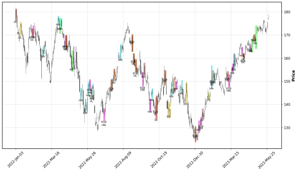
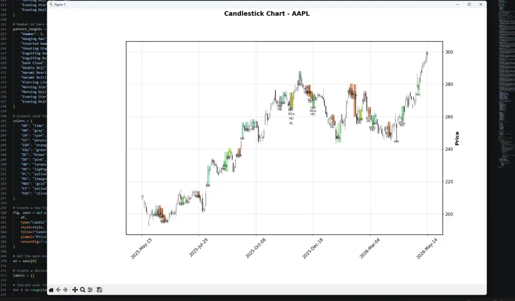
Hopefully you end up with a chart similar to mine below. The full chart is useful for checking that the scanner is running, the labels are being placed, and the highlighted boxes are appearing around the correct candles.
If we then zoom in a bit by using the magnifying glass in the bottom toolbar and drawing a rectangle over an area of interest we get:
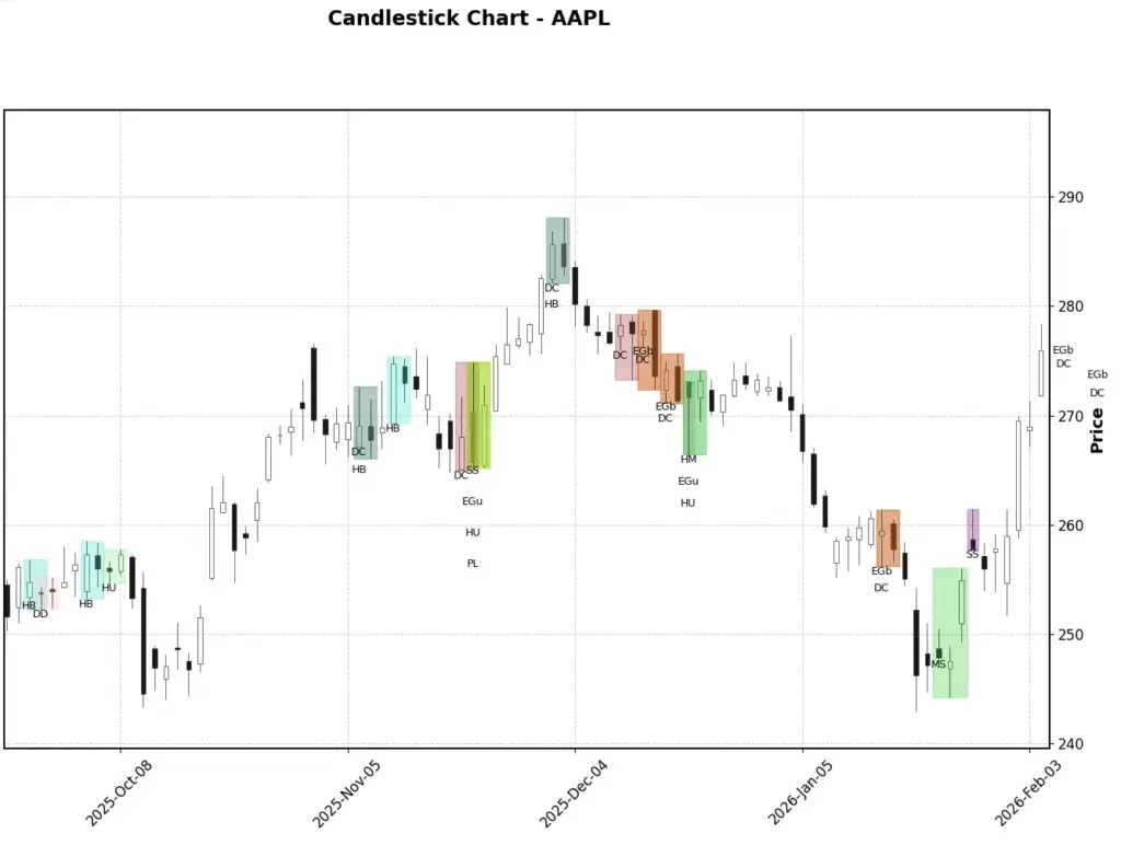
Zooming in makes the scanner output more useful. Around the early part of this section, the script picks up bearish or hesitation-style patterns such as Harami Bearish (HB) and Dark Cloud Cover (DC) near the top of the move. Later, during the pullback and recovery phase, the chart shows how several labels can appear close together when candles share similar bodies, shadows or gaps.
The Morning Star (MS) label near the start of the recovery in January 2026 in green, is a good example of the scanner doing what we want: it identifies a multi-candle formation and highlights the full pattern area rather than only the final candle. The subsequent purple Shooting Star (SS) label part way up the recovery also shows why context matters when reviewing scanner output. The code finds the candle shape; the trader still decides whether it matters for the chart being studied.
This is also why the label spacing matters. Without spacing, several labels can sit on top of each other and become unreadable. The simple 0.3 spacing used in the code keeps overlapping detections visible enough to inspect.
Next Steps for a Candlestick Pattern Scanner
Once the single-chart version is working, the obvious next step is to scan more than one ticker.
A simple scanner could loop through a watchlist, run the same pattern functions on each symbol, and save the most recent detections to a CSV file. That would let you check which stocks, futures, CFDs or ETFs have triggered formations without opening every chart manually.
You could also add filters. For example, you might only report bullish patterns after a recent decline, only show bearish patterns near resistance, or only keep patterns that appear with above-average volume.
The scanner can also be connected to alerts later. The basic version in this article is visual, but the same True/False pattern columns can be used to send an email, write to a file, or trigger a dashboard update.
Final Thoughts
This script gives you a working starting point for candlestick pattern recognition in Python. It downloads OHLC data, checks for one-bar, two-bar and three-bar formations, then marks the detected patterns directly on the chart.
From there, the interesting work is in testing what the detections actually mean. For example, you could check what happened 5 or 10 trading days after each bearish engulfing, hammer, harami, or evening star was detected. Did price continue in the expected direction, reverse, or simply chop sideways?
You can also compare candlestick detections against your other indicators. Do the patterns confirm an RSI, MACD, moving-average, or Bollinger Bands setup? Do they complement a congestion count indicator? That kind of follow-up is where the scanner becomes more useful than a visual chart label.
The first version here is deliberately visual if not pretty. It helps you see whether the pattern logic is firing where you expect. Once that is working, you can move toward backtesting, real-time scanning, alerts, or a larger portfolio watchlist.
Candlestick Pattern Reference Table
| Pattern Name | Pattern Type | Number of Bars | Pattern Description | Common Reading |
|---|---|---|---|---|
| Hammer | Bullish | Single | Small real body at the top, long lower shadow, short/no upper shadow. | Potential trend reversal, buying opportunity. |
| Hanging Man | Bearish | Single | Similar to Hammer but occurs at the end of an uptrend. | Possible top formation, selling opportunity. |
| Inverted Hammer | Bullish | Single | Small real body at the bottom, long upper shadow, short/no lower shadow. | Indicative of a potential trend reversal. |
| Shooting Star | Bearish | Single | Inverse of Inverted Hammer, appears in an uptrend. | Signals potential downward reversal. |
| Engulfing Bearish | Bearish | 2-Bar | A small bullish candle followed by a large bearish candle that engulfs the former. | Indicates a bearish reversal. |
| Engulfing Bullish | Bullish | 2-Bar | A small bearish candle followed by a large bullish candle that engulfs the former. | Suggests a bullish reversal. |
| Dark Cloud Cover | Bearish | 2-Bar | A bullish candle followed by a bearish candle that opens above the first’s high and closes below its midpoint. | Bearish reversal pattern in an uptrend. |
| Double Doji | Neutral or Bearish | 2-Bar | Two consecutive doji candles, where the open and close prices are almost the same. | Indicates indecision, potential for a reversal. |
| Harami Bearish | Bearish | 2-Bar | Large bullish candle followed by a smaller bearish candle within the previous body. | Signals a potential bearish reversal. |
| Harami Bullish | Bullish | 2-Bar | Large bearish candle followed by a smaller bullish candle within the previous body. | Suggests a potential bullish reversal. |
| Piercing Line | Bullish | 2-Bar | A bearish candle followed by a bullish candle that opens below the previous low and closes more than halfway into its body. | Indicates a bullish reversal in a downtrend. |
| Morning Star | Bullish | 3-Bar | A bearish candle followed by a short body candle and then a bullish candle. | Suggests a bullish reversal after a downtrend. |
| Morning Doji Star | Bullish | 3-Bar | Similar to Morning Star but with a Doji as the second candle. | Strong indicator of a bullish reversal. |
| Evening Star | Bearish | 3-Bar | A bullish candle followed by a short body candle and then a bearish candle. | Indicates a bearish reversal after an uptrend. |
| Evening Doji Star | Bearish | 3-Bar | Similar to Evening Star but with a Doji as the second candle. | Strong indicator of a bearish reversal. |
Further Reading
Japanese Candlestick Charting Techniques, Steve Nison.
Related AlphaSquawk guides:
RSI, for momentum confirmation.
Moving Averages, for trend context.
Bollinger Bands, for volatility and price-location context.
MACD, for moving-average momentum.
ADX, for trend-strength filtering.