Updated May 2026: I’ve refreshed this OBV guide with a clearer formula explanation, more detailed notes on divergence and volume confirmation, and an updated Python chart tutorial.

What Is On Balance Volume?
On Balance Volume, usually shortened to OBV, is a volume-based indicator that keeps a running total of volume.
The logic is straightforward. If price closes higher than the previous bar, that bar’s volume is added to OBV. If price closes lower, that bar’s volume is subtracted. If price closes unchanged, OBV stays the same.
The idea is to watch whether volume is supporting the price move. If price is rising and OBV is rising too, volume is broadly confirming the move. If price is rising but OBV is falling, the rally may be less convincing because volume is not moving with price.
I would not treat OBV as some sneaky early-warning system. It is still based on historical price and volume. It can help show accumulation, distribution and divergence, but the chart still needs context.
In this guide I’ll walk through where OBV came from, how the formula works, how traders read OBV trends and divergence, and how to calculate and plot OBV in Python.
Where OBV Comes From
OBV was introduced by Joseph Granville in his 1963 book Granville’s New Key to Stock Market Profits.
Granville’s basic belief was that volume often leads price. If volume starts building while price has not yet moved much, the market may be storing pressure before a larger move.
That “volume before price” idea is why traders still look at OBV. They are not only asking whether price is going up or down. They are asking whether volume is confirming the move, quietly disagreeing with it, or warning that something is changing under the surface.
This is also where some care is needed. OBV assigns the whole bar’s volume as positive or negative based only on whether the close rose or fell. That makes it easy to read, but it also means the indicator is fairly blunt.
How On Balance Volume Is Calculated
OBV is a cumulative indicator. It starts from an initial value, often zero, and then adds or subtracts each bar’s volume depending on whether the close rose or fell.
Before the formula, here are the symbols:
OBVₜ means the current OBV value.
OBVₜ₋₁ means the previous OBV value.
Vₜ means the current bar’s volume.
Cₜ means the current close.
Cₜ₋₁ means the previous close.
OBV_t =
\begin{cases}
OBV_{t-1} + V_t, & \text{if } C_t > C_{t-1} \\
OBV_{t-1} - V_t, & \text{if } C_t < C_{t-1} \\
OBV_{t-1}, & \text{if } C_t = C_{t-1}
\end{cases}
OBV adds volume on up closes, subtracts volume on down closes, and does nothing when the close is unchanged.
For example, if yesterday’s OBV was 1,000,000 and today closes higher on volume of 200,000, today’s OBV becomes 1,200,000.
If the next bar closes lower on volume of 150,000, OBV falls to 1,050,000.
The absolute OBV number is not usually the most important part. Because OBV is cumulative, its level depends on where the calculation started. Traders usually care more about the direction of the OBV line, trend breaks in OBV, and divergence between OBV and price.
This is why two charting platforms can show slightly different OBV levels while still showing the same useful behaviour. If they start the calculation from different dates, the raw number may differ, but the rises, falls and divergences should look similar.
How Traders Use OBV
OBV is mainly useful as a confirmation and divergence tool.
The first thing I look at is the direction of the OBV line. If price is rising and OBV is rising too, volume is broadly supporting the move. If price is rising but OBV is flat or falling, the rally may be weaker than it looks.
The same applies on the downside. If price is falling and OBV is falling too, volume is confirming the sell-off. If price is falling but OBV starts rising, downside pressure may be fading.
The second useful reading is divergence. A bullish OBV divergence appears when price makes a lower low but OBV makes a higher low. That can suggest selling pressure is weakening. A bearish OBV divergence appears when price makes a higher high but OBV makes a lower high. That can suggest the rally is not being backed by volume.
I would not treat OBV divergence as a trade by itself, but it can be a warning sign. Price still needs to confirm the turn.
Another practical use is watching OBV trend breaks. If OBV has been rising steadily and then breaks its own trendline before price does, it may be an early warning that participation is changing. The same can happen in reverse during a downtrend.
One caveat matters for forex and CFDs. Exchange-traded stocks and futures have clearer volume data. Spot FX does not have one central exchange, so many platforms use tick volume or broker-provided volume instead. OBV can still be useful there, but the quality of the volume input matters.
| OBV reading | What it shows | How I would read it |
|---|---|---|
| Price rising, OBV rising | Volume supports the rally | Bullish confirmation |
| Price rising, OBV falling | Volume does not confirm price | Possible bearish warning |
| Price falling, OBV falling | Volume supports the sell-off | Bearish confirmation |
| Price falling, OBV rising | Selling pressure may be fading | Possible bullish warning |
| OBV breaks its own trendline | Volume behaviour changes before price | Early warning, not a trigger |
| Large one-off volume spike | OBV may jump sharply | Check the news or event behind it |
OBV Strengths and Limitations
OBV is useful because it gives volume a direction. Instead of looking at volume bars one by one, the indicator builds a running line that rises when volume is attached to up closes and falls when volume is attached to down closes.
That makes OBV easy to compare with price. If both are moving in the same direction, volume is broadly confirming the trend. If they start to disagree, the divergence is worth investigating.
The weakness is that OBV is blunt. It assigns the full bar’s volume as positive or negative based only on whether the close rose or fell. It does not care where the close sits inside the day’s range. A tiny up close on huge volume is still added. A tiny down close on huge volume is still subtracted.
OBV can also be distorted by one-off volume spikes. Earnings, index rebalances, contract rolls, corporate actions, or sudden news can push the line sharply and make the next few readings harder to interpret.
The absolute OBV number is not usually the point. The trend, slope, divergence and breaks in the OBV line are usually more useful than the raw value.
| Strength | Why it helps |
|---|---|
| Simple calculation | Easy to understand and code |
| Combines price direction with volume | Shows whether volume is backing the move |
| Useful for divergence | Can warn when price and volume stop agreeing |
| Trend confirmation | Rising price plus rising OBV is cleaner than rising price alone |
| Works across timeframes | Can be used on daily, intraday or weekly charts where volume data is available |
| Weakness | Why it matters |
|---|---|
| Blunt volume treatment | All volume is added or subtracted based only on close direction |
| Sensitive to volume spikes | One event can distort the line |
| Arbitrary starting point | The absolute OBV value depends on where the calculation begins |
| Volume quality varies | Spot FX and CFD volume may not match exchange volume |
| Needs price context | OBV alone does not define entry, stop or target |
OBV vs Accumulation/Distribution Line and Other Volume Indicators
OBV is not the only volume-based indicator traders use. The closest comparison is the Accumulation/Distribution Line, because both try to turn price and volume into a running measure of buying or selling pressure.
Chaikin Money Flow is another useful comparison. CMF looks at where price closes inside the high-low range and weights that by volume over a lookback period. OBV is simpler: it only checks whether the close was higher or lower than the previous close, then adds or subtracts the full bar’s volume.
Money Flow Index takes a different route again. It combines price and volume into a bounded oscillator, so traders often read it more like a volume-weighted RSI.
Raw volume bars and volume moving averages are simpler still. They show how much activity occurred, but they do not give that activity a cumulative bullish or bearish direction by themselves.
| Indicator | Main input | What it tries to show | Main weakness |
|---|---|---|---|
| OBV | Close vs previous close + volume | Whether volume is accumulating on up closes or down closes | Ignores where price closed inside the bar |
| Accumulation/Distribution Line | Close location inside high-low range + volume | Whether volume is leaning toward accumulation or distribution | More complex and can disagree with OBV |
| Chaikin Money Flow | Money flow volume over a lookback period | Buying or selling pressure over recent bars | Can be distorted by gaps and close-location quirks |
| Money Flow Index | Typical price + volume | Volume-weighted momentum / stretched conditions | Can give false overbought or oversold readings in trends |
| Volume moving average | Raw volume smoothed over time | Whether activity is high or low versus normal | No directional signal by itself |
OBV Key Takeaways Before We Code
- OBV is a cumulative volume indicator.
- It adds volume when price closes higher and subtracts volume when price closes lower.
- The raw OBV value depends on the starting point, so the direction and shape of the line matter more than the absolute number.
- Rising price with rising OBV supports a bullish reading.
- Rising price with falling OBV can warn that volume is not confirming the move.
- Falling price with falling OBV supports a bearish reading.
- Falling price with rising OBV can warn that selling pressure may be fading.
- OBV divergence is useful, but it still needs price confirmation.
- Large volume spikes can distort OBV.
- OBV works best when the volume data is reliable, which is easier with exchange-traded stocks and futures than with decentralised spot FX.
- The Python tutorial below calculates OBV and plots it under a candlestick chart.
Coding OBV in Python and Plotting the Chart
Now we can build the On Balance Volume indicator in Python.
I am going to keep this as a step-by-step tutorial rather than dropping in one large script. Each Python-labelled block goes into the same file, in order. By the end, we will have downloaded market data, calculated OBV, and plotted it below a candlestick chart.
For this example I use SPY so the chart has clean daily price and exchange-volume data from Yahoo Finance. The same logic can be tested on other markets, but remember that volume quality varies. Exchange-traded stocks and futures usually have cleaner volume than decentralised spot FX or many CFD feeds.
Step 1: Install the Python libraries
python -m pip install yfinance pandas mplfinance matplotlibOn some Windows machines, this version works instead:
py -m pip install yfinance pandas mplfinance matplotlibStep 2: Create the file and import the libraries
Create a new Python file and save it as:
obv_indicator.py
At the top of the file, add:
import pandas as pd
import yfinance as yf
import mplfinance as mpf
from matplotlib.lines import Line2Dpandas stores the price data in a table and lets us calculate OBV.
yfinance downloads the market data.
mplfinance draws the candlestick chart.
Line2D lets us create a clean legend for the OBV line.
Step 3: Add the settings
Next, add a small settings section near the top of the file.
ticker = "SPY"
chart_title = "SPDR S&P 500 ETF"

start_date = "2025-05-01"
end_date = "2026-05-01"
ticker is the Yahoo Finance symbol.
chart_title is the title printed on the chart.
The dates use YYYY-MM-DD format. yfinance treats the end date as a cut-off, so you can push it one trading day later if you want the most recent available bar included.
Step 4: Download the market data
data = yf.download(
    ticker,
    start=start_date,
    end=end_date,
    auto_adjust=True,
    progress=False,
    multi_level_index=False
)

if data.empty:
    raise RuntimeError("No data was downloaded. Check the ticker symbol and date range.")

if isinstance(data.columns, pd.MultiIndex):
    data.columns = data.columns.get_level_values(0)

data.index = pd.DatetimeIndex(data.index)This downloads open, high, low, close and volume data.
auto_adjust=True keeps the price series adjusted where applicable.
progress=False removes the download progress bar.
multi_level_index=False keeps the columns easier to work with.
The final line makes sure the index is treated as dates, which mplfinance expects when plotting.
Step 5: Define the OBV function
def calculate_obv(data):
    close = data["Close"]
    volume = data["Volume"]

    obv = pd.Series(0, index=data.index, dtype="float64")

    for i in range(1, len(data)):
        if close.iloc[i] > close.iloc[i - 1]:
            obv.iloc[i] = obv.iloc[i - 1] + volume.iloc[i]
        elif close.iloc[i] < close.iloc[i - 1]:
            obv.iloc[i] = obv.iloc[i - 1] - volume.iloc[i]
        else:
            obv.iloc[i] = obv.iloc[i - 1]

return obvThe function checks each close against the previous close.
If the close is higher, that bar’s volume is added.
If the close is lower, that bar’s volume is subtracted.
If the close is unchanged, OBV stays where it was.
Step 6: Calculate OBV
Now call the function and add OBV to the data table.
data["OBV"] = calculate_obv(data)

plot_data = data.dropna(subset=["OBV"])Think of data as a spreadsheet. It already has Open, High, Low, Close and Volume columns. This step adds a new column called OBV.
Step 7: Define the OBV chart line
Next we tell mplfinance how to draw the OBV line below the price chart.
obv_plot = [
    mpf.make_addplot(
        plot_data["OBV"],
        panel=2,
        color="blue",
        width=1.2,
        ylabel="OBV"
    )
]panel=2 places OBV below the price and volume panels.
The blue line is the running OBV total.
Step 8: Create the chart
Now create the candlestick chart and add the OBV panel.
fig, axes = mpf.plot(
    plot_data,
    type="candle",
    style="yahoo",
    volume=True,
    addplot=obv_plot,
    panel_ratios=(3, 1, 1.4),
    title=f"{chart_title} with On Balance Volume",
    figsize=(11, 7),
    returnfig=True
)

fig.subplots_adjust(
    left=0.07,
    right=0.90,
    top=0.92,
    bottom=0.16,
    hspace=0.05
)type="candle" gives us the candlestick chart.
volume=True adds the volume panel.
addplot=obv_plot adds the OBV line.
panel_ratios controls the relative size of the price, volume and OBV panels.
subplots_adjust gives the chart extra room so the right-hand labels and angled dates are not clipped.
Step 9: Add the legend and show the chart
Finally, add a legend, save the image and show the chart.
obv_axis = axes[4] if len(axes) > 4 else axes[-1]

legend_items = [
    Line2D([], [], color="blue", label="OBV")
]

obv_axis.legend(handles=legend_items, loc="upper left")

fig.savefig("obv_indicator_chart.png", dpi=150, bbox_inches="tight")

mpf.show()fig.savefig() saves the chart as a PNG image in the same folder as the script.
mpf.show() opens the chart window.
Step 10: Run the script
Save obv_indicator.py by pressing Ctrl+S.
The easiest route is usually to click the play button in the top-right corner of VS Code. If that works, the chart window should open.
You can also run it from the terminal. Open Terminal > New Terminal, move into the folder where you saved the script, then run:
python obv_indicator.pyOn some Windows setups, use:
py obv_indicator.pyYour chart should show SPY candlesticks at the top, volume underneath, and an OBV panel below that. The exact shape will depend on the ticker and date range you choose but should look something like mine seen below:
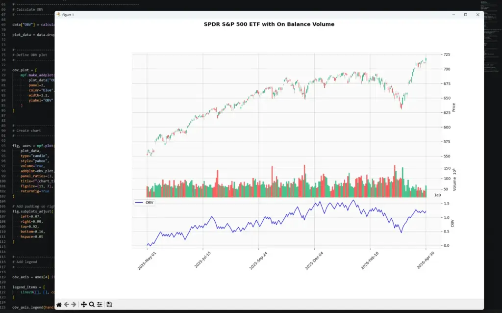
In this example, OBV broadly confirms the earlier advance because the line rises with price. Later, after the sharp pullback and recovery, price pushes toward new highs while OBV is still below its earlier peak. That does not automatically mean the rally must fail, but it is the kind of non-confirmation OBV traders would notice.
If you want to double check your result, bring up the same chart and timeframe on say, Yahoo Finance website and add the OBV indicator to it. I can confirm their OBV line looks identical in behaviour to what we have here.
Once the script works, start changing the inputs.
To change the market, edit:
ticker = "SPY"
chart_title = "SPDR S&P 500 ETF"To change the date range, edit:
start_date = "2025-05-01"
end_date = "2026-05-01"Try the script on a liquid stock, ETF or futures proxy first. If you use it on forex or CFDs, check what kind of volume your data source is actually providing. Spot FX platforms often use tick volume rather than centralised exchange volume.
Further Reading
For the original OBV source, start with Granville’s book. For practical comparison, it is also worth reading up on the Accumulation/Distribution Line and other volume-based indicators like Chaikin Money Flow.
Granville, J. (1963). Granville’s New Key to Stock Market Profits. Prentice-Hall.