Fast Stochastics Indicator: Formula, Settings, Signals & Python

Updated May 2026: I’ve refreshed this guide with clearer Fast Stochastics formulas, more practical notes on settings and signals, a comparison with Slow Stochastics, and an updated Python walkthrough.

• Email this Page
• Share on Facebook
• Share on Reddit
• Share on WhatsApp
• Share on Telegram
• Email this Page

What Is the Fast Stochastics Indicator?

Fast Stochastics is a momentum oscillator that shows where the latest close sits inside a recent high-low range.

That is the key idea. The indicator does not measure speed directly. It asks whether price is closing near the top of its recent range, near the bottom of its recent range, or somewhere in the middle.

If the close is near the top of the range, Fast Stochastics rises toward the upper end of its scale. If the close is near the bottom of the range, it falls toward the lower end. The scale runs from 0 to 100.

Fast Stochastics has two main lines. %K is the faster line and shows the close’s position inside the recent range. %D is a moving average of %K.

Fast refers to the indicator’s responsiveness compared with Slow Stochastics. That can be useful for short-term traders, but it also means more whipsaws. A fast signal is not necessarily a better signal.

Fast Stochastics at a Glance

Fast Stochastics has a simple job.

It compares the current close with the highest high and lowest low over a chosen lookback period.

If price closes near the recent high, %K moves higher.

If price closes near the recent low, %K moves lower.

%D then smooths %K with a short moving average.

Traders often watch the 80 and 20 levels. Readings above 80 are commonly called overbought. Readings below 20 are commonly called oversold. Those are context zones, not definitive trade instructions.

I would read Fast Stochastics as a range-position tool. It shows whether price is closing near the top or bottom of its recent range; the chart decides whether that means trend strength, exhaustion, or noise.

Fast Stochastics and George Lane

The stochastic oscillator is usually associated with George C. Lane, who introduced the indicator in the 1950s. Fast Stochastics is the more responsive version of the stochastic oscillator and is close to the original form traders encountered before slower, more smoothed versions became common.

The indicator is built around closing location. In a strong upward move, price often closes near the upper part of its recent high-low range. In a weak move, price often closes near the lower part of that range.

Fast Stochastics reacts quickly to those shifts. That is useful for short-term traders who want earlier signals, but it also means the lines can whip around in choppy markets.

Slow Stochastics adds extra smoothing, which makes the indicator less jumpy but slower to react. That is why Fast Stochastics is often used when responsiveness matters, while Slow Stochastics may be preferred when the trader wants fewer signals and less noise.

Fast Stochastics Formula

Fast Stochastics is built from two lines: %K and %D.

%K is the faster line. It measures where the current close sits inside the recent high-low range.

%D is the slower signal line. It is a moving average of %K.

The usual scale runs from 0 to 100. A high reading means price is closing near the top of the recent range. A low reading means price is closing near the bottom of the recent range.

Formula Key

1. Find the recent high-low range

First, choose the lookback period. A common setting is 14 bars, but the formula works on any chart timeframe.

The high-low range is the distance between the highest high and lowest low over that lookback period.

\text{Range}_t = HH(n)_t - LL(n)_t

The range equals the highest high over the lookback period minus the lowest low over the same period.

2. Calculate Fast %K

Fast %K measures where the current close sits inside that recent range.

\%K_t = 100 \times \frac{C_t - LL(n)_t}{HH(n)_t - LL(n)_t}

Fast %K equals the current close minus the lowest low, divided by the highest high minus the lowest low, multiplied by 100.

If the close is near the top of the range, %K will be high. If the close is near the bottom of the range, %K will be low.

3. Calculate Fast %D

Fast %D is a moving average of Fast %K. The common setting is a 3-period average.

\%D_t = MA_m(\%K_t)

Fast %D is the moving average of Fast %K over the chosen smoothing period.

With a 3-period %D, the line smooths the last three %K values.

Original vs simplified Fast %D

Some platforms distinguish between an original and a simplified Fast Stochastics calculation.

In the simplified version, the closing-range ratio is calculated first, then smoothed.

In the original version, the closing range and total range are smoothed separately before the division is made.

For most traders, the important point is practical rather than theoretical. Check which algorithm your charting platform uses if you are trying to match values exactly across platforms.

The formula explains why Fast Stochastics can be jumpy. It reacts whenever the close moves toward the top or bottom of the recent range. That responsiveness is useful, but it can also create false turns in choppy markets.

This is also why Fast Stochastics and Slow Stochastics can give different-looking signals. Slow Stochastics adds more smoothing, while Fast Stochastics keeps the raw range-position signal closer to the surface.

How to Interpret Fast Stochastics Signals

Fast Stochastics signals are easiest to understand once you remember what the indicator measures.

It does not tell you that price is “fast” in the usual sense. It tells you where the latest close sits inside the recent high-low range.

A high reading means price is closing near the top of that range. A low reading means price is closing near the bottom. Whether that is bullish, bearish, overextended, or simply noisy depends on the chart around it.

The 80 and 20 levels are reference zones, not trading commands. A move above 80 is often called overbought, but in a strong trend price can keep closing near the top of its range for a long time. A move below 20 is often called oversold, but in a weak market price can keep closing near the bottom of its range.

The %K and %D crossover is also best treated as a warning or confirmation rather than a complete trade signal. A bullish crossover below 20 may matter if price is holding support or recovering from a failed breakdown. A bearish crossover above 80 may matter if price is failing at resistance or losing upside follow-through.

In the middle of a choppy range, the same cross can be almost meaningless. Fast Stochastics reacts quickly, so it can produce a lot of signals when price is not really going anywhere.

The safer habit is to read Fast Stochastics as a range-position oscillator. It shows whether price is closing high or low within its recent range. It does not know whether the market is trending, whether a breakout is real, or whether the next candle offers a good trade. Price structure still has to answer those questions.

Fast Stochastics Settings and Parameters

The common Fast Stochastics setup is a 14-period lookback for %K and a 3-period moving average for %D.

The lookback period controls the range being measured. A 14-period %K asks where the current close sits inside the highest high and lowest low of the last 14 bars.

The %D period controls how much the fast %K line is smoothed. A 3-period %D is common because it keeps the signal line responsive while removing some of the raw %K noise.

The word period simply means the chart bar being used. On a daily chart, 14 periods means 14 trading days. On a five-minute chart, it means 14 five-minute candles.

There is no single best setting for Fast Stochastics. The right setup depends on the market, timeframe and strategy.

A shorter %K lookback, such as 5 or 9 periods, will react faster. That can suit short-term trading, but it also creates more whipsaws.

A longer %K lookback, such as 21 or 28 periods, will react more slowly. That can reduce noise, but it may also make signals arrive late.

The same logic applies to %D smoothing. A shorter %D keeps the signal line close to %K. A longer %D smooths the signal more, but the crossover may happen later.

I would start with the standard 14 and 3 setup, then compare changes against that baseline. Changing the settings just to make old signals look cleaner can create a curve-fitted indicator that fails when the market changes.

Fast Stochastics Strategy Examples

A Fast Stochastics strategy should start with the market condition.

The same oscillator signal can mean different things in a trend and in a range. In a strong uptrend, repeated moves above 80 can show persistent buying pressure. In a sideways range, a move above 80 may warn that price is stretched near the top of the range.

That is why I would separate Fast Stochastics strategies into a few practical groups.

A bullish continuation setup might use Fast Stochastics after a pullback. If price holds a higher low and %K turns back above %D, the crossover may support the idea that momentum is returning. The signal is stronger if price is also holding above a clear support level or moving average.

A bearish continuation setup works the other way. If price fails at resistance, forms a lower high, and %K crosses below %D, the signal may support a short-side view.

For mean reversion, I would be more selective. A move below 20 is not enough by itself. I would want to see price at support, a failed breakdown, or a clear loss of downside follow-through. A move above 80 is not enough by itself either. I would want resistance, a failed breakout, or weakening price action.

The main thing I would avoid is trading every %K and %D cross. Fast Stochastics is designed to react quickly, so it will often turn before a slower indicator does. That responsiveness is useful, but it also means the indicator can produce plenty of weak signals when price is chopping around.

Fast Stochastics vs Slow Stochastics

Fast Stochastics and Slow Stochastics are built from the same basic idea: where does the close sit inside the recent high-low range?

The difference is smoothing.

Fast Stochastics keeps the raw %K line closer to the surface. It reacts quickly when price closes near the top or bottom of the range.

Slow Stochastics smooths the signal more. That makes it less jumpy, but slower to react.

This is why the “best” version depends on the job. Fast Stochastics may suit short-term traders who want earlier warnings. Slow Stochastics may suit traders who prefer fewer signals and a cleaner oscillator.

A fast signal is not automatically better. Earlier signals are useful only if they improve the trade decision. If they mostly create extra false starts, the slower version may be better.

A slow signal is not automatically safer either. It can keep the trader out of some noise, but it may also confirm the move after the better entry has already passed.

I would compare the two versions on the same market and timeframe before choosing one. Watch how often each version crosses, how often the cross leads to a useful move, and how often it simply reacts to noise.

I would avoid treating Fast and Slow Stochastics as completely different indicators. They are two versions of the same range-position idea. The main choice is how much smoothing you want between the raw signal and the trade decision.

Pros and Cons of Fast Stochastics

Fast Stochastics is useful because it reacts quickly when price starts closing near the top or bottom of its recent range.

That responsiveness is the main appeal. It can help short-term traders spot changes in range position before slower, more smoothed indicators react. The problem is that the same responsiveness can also create weak signals in choppy markets.

The limitations come from the same feature. Fast Stochastics can turn quickly, but it can also turn too often.

A reading above 80 does not force price to reverse. It may simply show that price keeps closing near the top of its range during an uptrend. A reading below 20 does not force price to bounce. It may show persistent downside pressure.

Crossovers can also be noisy. In a sideways market, %K and %D may cross repeatedly without price making useful progress.

Used well, Fast Stochastics can help judge whether price is closing strongly or weakly inside a recent range. Used badly, it can tempt traders into taking every crossover and fading every overbought or oversold reading.

Coding Fast Stochastics with Python

Now we can calculate Fast Stochastics in Python and plot it under a candlestick chart.

The code follows the formula from above. It finds the highest high and lowest low over the lookback period, calculates %K, then calculates %D as a moving average of %K.

The example below downloads price data, calculates Fast Stochastics with a 14-period %K and 3-period %D, then plots price, volume, %K and %D in separate panels.

Step 1: Install the Python libraries

python -m pip install pandas yfinance numpy matplotlib mplfinance

python -m pip install pandas yfinance numpy matplotlib mplfinance

If your Windows setup uses the py launcher, this version may work better:

py -m pip install pandas yfinance numpy matplotlib mplfinance

py -m pip install pandas yfinance numpy matplotlib mplfinance

Pandas handles the data table, yfinance downloads the price data, NumPy helps with the calculations, matplotlib builds the chart, and mplfinance provides the candlestick plotting function.

Step 2: Create the file and import the libraries

Save a new file as fast_stochastics.py, then paste the following imports at the top.

import numpy as np
import pandas as pd
import yfinance as yf
import matplotlib.pyplot as plt
from mplfinance.original_flavor import candlestick_ohlc

import numpy as np
import pandas as pd
import yfinance as yf
import matplotlib.pyplot as plt
from mplfinance.original_flavor import candlestick_ohlc

Step 3: Add the chart settings

ticker = "BABA"
start_date = "2025-05-13"
end_date = "2026-05-13"

k_period = 14
d_period = 3

ticker = "BABA"
start_date = "2025-05-13"
end_date = "2026-05-13"

k_period = 14
d_period = 3

This example uses Alibaba with a 14-period Fast %K and a 3-period Fast %D. The same script can be reused with another ticker, date range or setting by changing these values.

Step 4: Download the price data

data = yf.download(
    ticker,
    start=start_date,
    end=end_date,
    auto_adjust=True,
    progress=False,
    multi_level_index=False
)

if isinstance(data.columns, pd.MultiIndex):
    data.columns = data.columns.get_level_values(0)

data.index = pd.DatetimeIndex(data.index)
data = data.dropna(subset=["Open", "High", "Low", "Close", "Volume"])

if data.empty:
    raise ValueError("No price data downloaded. Check the ticker and date range.")

data = yf.download(
    ticker,
    start=start_date,
    end=end_date,
    auto_adjust=True,
    progress=False,
    multi_level_index=False
)

if isinstance(data.columns, pd.MultiIndex):
    data.columns = data.columns.get_level_values(0)

data.index = pd.DatetimeIndex(data.index)
data = data.dropna(subset=["Open", "High", "Low", "Close", "Volume"])

if data.empty:
    raise ValueError("No price data downloaded. Check the ticker and date range.")

The auto_adjust=True setting means the OHLC data is adjusted for splits and dividends. The MultiIndex fallback is included because yfinance can return multi-level columns depending on version and settings.

Step 5: Define the Fast Stochastics calculation

def calculate_fast_stochastics(price_data, k_period=14, d_period=3):
    df = price_data.copy()

    lowest_low = df["Low"].rolling(window=k_period).min()
    highest_high = df["High"].rolling(window=k_period).max()

    price_range = highest_high - lowest_low

    df["Fast_%K"] = np.where(
        price_range != 0,
        100 * (df["Close"] - lowest_low) / price_range,
        np.nan
    )

    df["Fast_%D"] = df["Fast_%K"].rolling(window=d_period).mean()

    return df

def calculate_fast_stochastics(price_data, k_period=14, d_period=3):
    df = price_data.copy()

    lowest_low = df["Low"].rolling(window=k_period).min()
    highest_high = df["High"].rolling(window=k_period).max()

    price_range = highest_high - lowest_low

    df["Fast_%K"] = np.where(
        price_range != 0,
        100 * (df["Close"] - lowest_low) / price_range,
        np.nan
    )

    df["Fast_%D"] = df["Fast_%K"].rolling(window=d_period).mean()

    return df

The price_range check avoids dividing by zero if the high and low are identical over the lookback window. That is uncommon in liquid markets, but it is safer to handle it.

Step 6: Add the Fast Stochastics columns

data = calculate_fast_stochastics(
    data,
    k_period=k_period,
    d_period=d_period
)

plot_data = data.dropna(subset=["Fast_%K", "Fast_%D"]).copy()

if plot_data.empty:
    raise ValueError("Not enough valid data to calculate Fast Stochastics.")

data = calculate_fast_stochastics(
    data,
    k_period=k_period,
    d_period=d_period
)

plot_data = data.dropna(subset=["Fast_%K", "Fast_%D"]).copy()

if plot_data.empty:
    raise ValueError("Not enough valid data to calculate Fast Stochastics.")

The first rows are removed because the rolling high-low range and %D moving average need enough bars before they can be calculated.

Step 7: Prepare the chart data

plot_data["Bar"] = np.arange(len(plot_data))

ohlc = plot_data[["Bar", "Open", "High", "Low", "Close"]].values

volume_colors = np.where(
    plot_data["Close"] >= plot_data["Open"],
    "green",
    "red"
)

plot_data["Bar"] = np.arange(len(plot_data))

ohlc = plot_data[["Bar", "Open", "High", "Low", "Close"]].values

volume_colors = np.where(
    plot_data["Close"] >= plot_data["Open"],
    "green",
    "red"
)

This prepares the candlestick and volume data for the chart.

Step 8: Create the price, volume and Fast Stochastics panels

fig, (ax_price, ax_volume, ax_stoch) = plt.subplots(
    3,
    1,
    figsize=(12, 7),
    sharex=True,
    gridspec_kw={
        "height_ratios": [4, 1, 1.4],
        "hspace": 0.0
    }
)

fig.suptitle(
    f"{ticker} with Fast Stochastics ({k_period}, {d_period})",
    fontsize=12,
    fontweight="bold"
)

candlestick_ohlc(
    ax_price,
    ohlc,
    width=0.6,
    colorup="green",
    colordown="red",
    alpha=0.85
)

ax_price.set_ylabel("Price")
ax_price.grid(True, alpha=0.25)

ax_volume.bar(
    plot_data["Bar"],
    plot_data["Volume"],
    color=volume_colors,
    width=0.6,
    alpha=0.55
)

ax_volume.set_ylabel("Volume")
ax_volume.grid(True, alpha=0.25)

ax_stoch.plot(
    plot_data["Bar"],
    plot_data["Fast_%K"],
    label="Fast %K",
    color="blue",
    linewidth=1.1
)

ax_stoch.plot(
    plot_data["Bar"],
    plot_data["Fast_%D"],
    label="Fast %D",
    color="brown",
    linewidth=1.3
)

ax_stoch.axhline(80, color="gray", linestyle="--", linewidth=1.0, alpha=0.8)
ax_stoch.axhline(20, color="gray", linestyle="--", linewidth=1.0, alpha=0.8)
ax_stoch.axhline(50, color="black", linestyle=":", linewidth=0.8, alpha=0.7)

ax_stoch.text(
    1.002, 80, "80",
    transform=ax_stoch.get_yaxis_transform(),
    va="center",
    fontsize=8,
    color="gray"
)

ax_stoch.text(
    1.002, 50, "50",
    transform=ax_stoch.get_yaxis_transform(),
    va="center",
    fontsize=8,
    color="black"
)

ax_stoch.text(
    1.002, 20, "20",
    transform=ax_stoch.get_yaxis_transform(),
    va="center",
    fontsize=8,
    color="gray"
)

ax_stoch.set_ylabel("Fast Stoch")
ax_stoch.set_ylim(0, 100)
ax_stoch.legend(loc="upper left", fontsize=8)
ax_stoch.grid(True, alpha=0.25)

fig, (ax_price, ax_volume, ax_stoch) = plt.subplots(
    3,
    1,
    figsize=(12, 7),
    sharex=True,
    gridspec_kw={
        "height_ratios": [4, 1, 1.4],
        "hspace": 0.0
    }
)

fig.suptitle(
    f"{ticker} with Fast Stochastics ({k_period}, {d_period})",
    fontsize=12,
    fontweight="bold"
)

candlestick_ohlc(
    ax_price,
    ohlc,
    width=0.6,
    colorup="green",
    colordown="red",
    alpha=0.85
)

ax_price.set_ylabel("Price")
ax_price.grid(True, alpha=0.25)

ax_volume.bar(
    plot_data["Bar"],
    plot_data["Volume"],
    color=volume_colors,
    width=0.6,
    alpha=0.55
)

ax_volume.set_ylabel("Volume")
ax_volume.grid(True, alpha=0.25)

ax_stoch.plot(
    plot_data["Bar"],
    plot_data["Fast_%K"],
    label="Fast %K",
    color="blue",
    linewidth=1.1
)

ax_stoch.plot(
    plot_data["Bar"],
    plot_data["Fast_%D"],
    label="Fast %D",
    color="brown",
    linewidth=1.3
)

ax_stoch.axhline(80, color="gray", linestyle="--", linewidth=1.0, alpha=0.8)
ax_stoch.axhline(20, color="gray", linestyle="--", linewidth=1.0, alpha=0.8)
ax_stoch.axhline(50, color="black", linestyle=":", linewidth=0.8, alpha=0.7)

ax_stoch.text(
    1.002, 80, "80",
    transform=ax_stoch.get_yaxis_transform(),
    va="center",
    fontsize=8,
    color="gray"
)

ax_stoch.text(
    1.002, 50, "50",
    transform=ax_stoch.get_yaxis_transform(),
    va="center",
    fontsize=8,
    color="black"
)

ax_stoch.text(
    1.002, 20, "20",
    transform=ax_stoch.get_yaxis_transform(),
    va="center",
    fontsize=8,
    color="gray"
)

ax_stoch.set_ylabel("Fast Stoch")
ax_stoch.set_ylim(0, 100)
ax_stoch.legend(loc="upper left", fontsize=8)
ax_stoch.grid(True, alpha=0.25)

The Fast Stochastics panel includes %K, %D, the common 80 and 20 reference zones, and a 50 midpoint line. The reference levels are labelled directly on the right so the legend can stay focused on %K and %D.

Step 9: Add date labels, save and show the chart

tick_count = 9
tick_positions = np.linspace(0, len(plot_data) - 1, tick_count, dtype=int)
tick_labels = plot_data.index[tick_positions].strftime("%Y-%m-%d")

ax_stoch.set_xticks(tick_positions)
ax_stoch.set_xticklabels(tick_labels, rotation=45, ha="right")

plt.setp(ax_price.get_xticklabels(), visible=False)
plt.setp(ax_volume.get_xticklabels(), visible=False)

fig.subplots_adjust(
    top=0.90,
    bottom=0.16,
    left=0.08,
    right=0.94,
    hspace=0.0
)

output_file = "fast_stochastics_python_chart.png"
fig.savefig(output_file, dpi=150, bbox_inches="tight")

print(f"Saved chart as {output_file}")

plt.show()

tick_count = 9
tick_positions = np.linspace(0, len(plot_data) - 1, tick_count, dtype=int)
tick_labels = plot_data.index[tick_positions].strftime("%Y-%m-%d")

ax_stoch.set_xticks(tick_positions)
ax_stoch.set_xticklabels(tick_labels, rotation=45, ha="right")

plt.setp(ax_price.get_xticklabels(), visible=False)
plt.setp(ax_volume.get_xticklabels(), visible=False)

fig.subplots_adjust(
    top=0.90,
    bottom=0.16,
    left=0.08,
    right=0.94,
    hspace=0.0
)

output_file = "fast_stochastics_python_chart.png"
fig.savefig(output_file, dpi=150, bbox_inches="tight")

print(f"Saved chart as {output_file}")

plt.show()

The script saves the chart as fast_stochastics_python_chart.png and opens the chart window.

Step 10: Run the script

Run the file from VS Code, or use this command in the terminal:

python fast_stochastics.py

python fast_stochastics.py

If your Windows setup uses the py launcher, use:

py fast_stochastics.py

py fast_stochastics.py

You should get a three-panel chart with price, volume, and Fast Stochastics. The oscillator panel shows how %K and %D move between the 0 and 100 range as price closes near the top or bottom of its recent high-low range.

Hopefully it looks something like the one I made below:

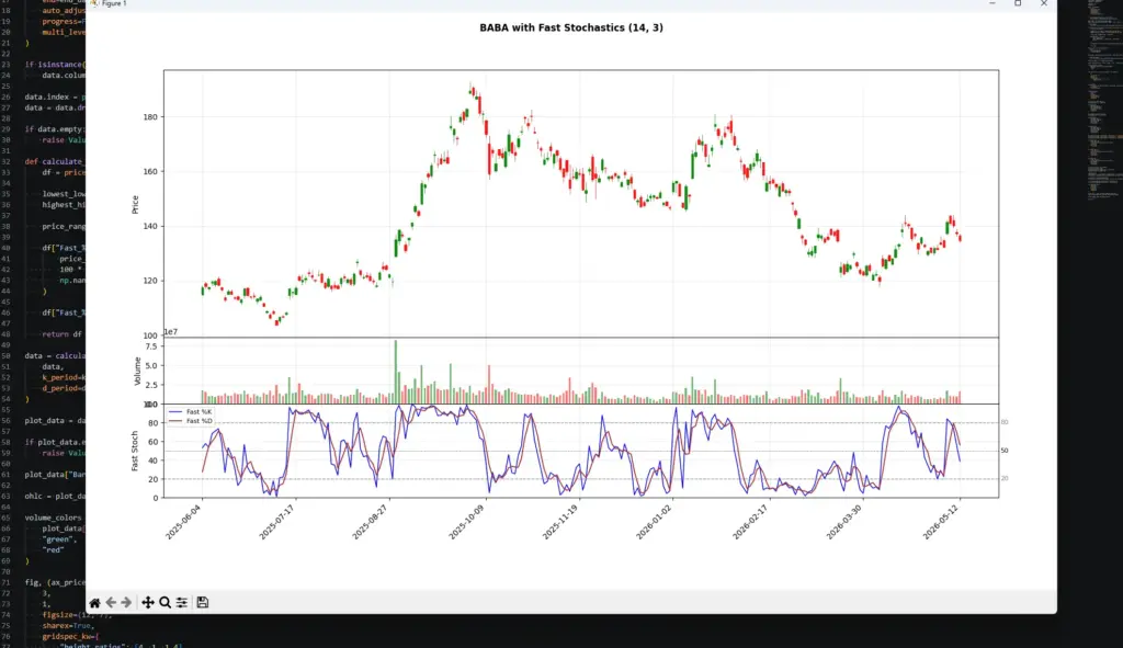
The chart shows why Fast Stochastics needs trend context. During the strong rally into autumn, %K and %D spend long stretches near or above 80 while price continues higher, so the upper-zone readings look more like momentum strength than automatic sell signals.

The later selloff shows the opposite problem. Stochastics falls sharply toward the lower zone as price weakens, but oversold readings alone would not have been enough to call a bottom. The useful clues come when the oscillator turns at the same time price starts to stabilise or reject a level.

On the right side of the chart, price has bounced from the spring lows, while Fast Stochastics has already moved back down from the upper zone. That is a good example of the indicator’s speed: it can warn that upside follow-through is fading early, but the chart still has to confirm whether that becomes a reversal, a pause, or just noise inside a recovery.

The chart ends before a later sharp move higher, which is another reminder that stochastic readings can change quickly after earnings or major news. The indicator can show range position, but it cannot know a catalyst is about to reprice the stock.

Fast Stochastics vs RSI, MACD and Bollinger Bands

Fast Stochastics works best when it has a clear job. It shows where the close sits inside a recent high-low range.

Other indicators answer different questions. RSI measures momentum on a 0 to 100 scale. MACD tracks moving-average momentum. Bollinger Bands show price relative to a volatility envelope. Volume helps check whether participation supports the move.

The mistake is adding indicators just because they are popular. A better approach is to decide what each tool contributes.

A common pairing is trend plus timing. For example, a trader might use a moving average or MACD to decide whether the broader chart is bullish or bearish, then use Fast Stochastics to watch for pullbacks or short-term turns.

For range trading, Bollinger Bands or support and resistance can help define where price is stretched. Fast Stochastics can then show whether price is also closing near the top or bottom of its recent range.

The cleaner approach is to give each tool a job. Fast Stochastics can help with timing, but it should not be forced to define the whole trade by itself.

Frequently Asked Questions about Fast Stochastics

Q: What is Fast Stochastics?

Fast Stochastics is a momentum oscillator that shows where the latest close sits inside a recent high-low range.

Q: What is the Fast Stochastics formula?

Fast %K equals the current close minus the lowest low, divided by the highest high minus the lowest low, multiplied by 100. Fast %D is a moving average of Fast %K.

Q: What is the difference between %K and %D?

%K is the faster line. It shows the close’s position inside the recent range. %D is a moving average of %K and acts as a smoother signal line.

Q: What are common Fast Stochastics settings?

A common setup is 14 periods for %K and 3 periods for %D. Shorter settings react faster. Longer or more smoothed settings reduce noise but react later.

Q: What does Fast Stochastics above 80 mean?

A reading above 80 means price is closing near the top of its recent range. In a range, that can warn of overextension. In an uptrend, it can show strength.

Q: What does Fast Stochastics below 20 mean?

A reading below 20 means price is closing near the bottom of its recent range. In a range, that can warn of downside overextension. In a downtrend, it can show persistent weakness.

Q: Is a %K and %D crossover a buy or sell signal?

Not by itself. A %K cross above %D can support a bullish view, and a cross below %D can support a bearish view, but the signal still needs price context.

Q: Is Fast Stochastics better than Slow Stochastics?

Fast Stochastics is more responsive. Slow Stochastics is smoother. Fast may suit short-term timing, while Slow may suit traders who want fewer noisy signals.

Q: Can Fast Stochastics be used for day trading?

Yes, but it can be noisy on short timeframes. I would use it as a timing and range-position tool, not as a mechanical entry system.

Final Thoughts

Fast Stochastics is simple once the formula is stripped back. It shows whether price is closing near the top or bottom of its recent high-low range.

That makes it useful for short-term timing, pullbacks, failed moves and range rotation. The trade-off is noise. Fast Stochastics can react early, but it can also react too often.

The 80 and 20 levels are reference zones, not instructions. A high reading can show strength in an uptrend. A low reading can show weakness in a downtrend. Crossovers also need price structure before they become useful.

I would treat Fast Stochastics as a quick range-position oscillator. It can help with timing, but the trade still needs trend context, support or resistance, risk control and awareness of market conditions.

Further Reading

Related AlphaSquawk guides:

Slow Stochastics, for the smoother version of the stochastic oscillator.

RSI, for another 0 to 100 momentum oscillator.

MACD, for moving-average momentum and crossover signals.

Bollinger Bands, for volatility bands around price.

Moving Averages, for trend direction and baseline filtering.

Parabolic SAR, for a price-based stop-and-reversal tool.

Average True Range, for volatility and stop-distance context.

Books and references:

Technical Analysis Explained, Martin J. Pring.

New Trading Systems and Methods, Perry Kaufman.

Technical Analysis from A to Z by Steven B. Achelis

Technical Analysis of the Financial Markets by John J. Murphy

The Encyclopedia of Technical Market Indicators by Robert W. Colby