Kalman Filter Trading: Python, Signals, Mean Reversion & Trend Smoothing

Updated May 2026: I’ve refreshed this guide with a clearer explanation of Kalman filter trading, practical notes on smoothing, mean reversion and signal use, and an updated Python walkthrough.

• Email this Page
• Share on Facebook
• Share on Reddit
• Share on WhatsApp
• Share on Telegram
• Email this Page

What Is a Kalman Filter in Trading?

A Kalman filter is a mathematical method for estimating an underlying state from noisy observations.

In trading, the noisy observation is often price. The underlying state might be a smoother trend estimate, a fair-value proxy inside a model, a dynamic hedge ratio, or another hidden variable the trader is trying to estimate.

Picture that price jumps around. Some of that movement may be useful information, and some may be noise. A Kalman filter tries to update its estimate as each new observation arrives, while deciding how much trust to place in the new data versus the previous estimate.

That makes it different from a normal moving average. A moving average applies a fixed smoothing rule, whereas a Kalman filter uses a prediction-and-update process, so the estimate can adapt as new observations arrive.

For trading, I would treat the Kalman filter as a model-based smoothing and estimation tool. It can help organise noisy price data, but it does not know the true value of a stock or derivative, future price, or hidden market intention. The output is only as good as the model, the assumptions and the noise settings.

Kalman Filter at a Glance

A Kalman filter works in two broad steps.

First, it predicts the current state from the previous state.

Second, it updates that prediction after seeing the latest observation.

In a trading chart, this often means estimating a smoother line from noisy price data. If the filter trusts new observations more, the line reacts faster but becomes noisier. If it trusts the prior estimate more, the line becomes smoother but reacts later.

That trade-off is the heart of using a Kalman filter in trading. More smoothing can make the chart easier to read, but it can also delay signals. Faster reaction can help catch turns earlier, but it can also follow noise.

So instead of questioning whether the Kalman filter is “right” it might be better to ask whether its estimate is useful for the strategy being tested.

Where the Kalman Filter Came From

The Kalman filter is named after Rudolf E. Kálmán, a Hungarian-American electrical engineer and mathematician who introduced the method in the context of linear filtering and prediction problems. It was published in his paper, “A New Approach to Linear Filtering and Prediction Problems” in 1960.

Its early use was not stock trading. The basic problem was how to estimate the state of a moving system when the measurements are noisy. That is why the method became important in control theory, navigation, tracking and signal processing before traders adapted the idea to markets.

The connection to trading is easy to see. Market prices are noisy observations. Traders often want a cleaner estimate of trend, value, volatility, or the relationship between two instruments. A Kalman filter gives a structured way to update that estimate as new data arrives.

The important caveat is that financial markets are not controlled engineering systems. Price behaviour can change because of earnings, liquidity, positioning, macro news or regime shifts. A Kalman filter can adapt to new observations, but it cannot remove uncertainty from the market.

Kalman Filter Formula Without Getting Lost

A Kalman filter works by repeating two steps.

First, it makes a prediction about the current state.

Second, it updates that prediction after seeing the latest observation.

In trading, the observation might be the latest price. The state might be a smoother estimate of the underlying trend. The filter keeps asking how much it should trust the new price compared with the previous estimate.

That is why the Kalman filter is often useful for noisy markets. It does not simply average the last few prices. It updates an estimate while also tracking how uncertain that estimate is.

Formula Key

1. Prediction step

The prediction step estimates where the state should be before the latest observation is used. In a trading example, this is the model’s estimate before it looks at the newest price.

\hat{x}_{k|k-1} = F_k \hat{x}_{k-1|k-1} + B_k u_k

The predicted state equals the previous updated state passed through the transition model, plus any control input.

The filter also predicts how uncertain that estimate is.

P_{k|k-1} = F_k P_{k-1|k-1} F_k^\top + Q_k

The predicted uncertainty comes from the previous uncertainty, adjusted by the transition model, plus process noise.

2. Kalman gain

The Kalman gain decides how much weight the filter gives to the new observation.

If the filter trusts the new observation more, the estimate reacts faster. If it trusts the previous estimate more, the line becomes smoother but slower.

K_k = P_{k|k-1} H_k^\top \left(H_k P_{k|k-1} H_k^\top + R_k\right)^{-1}

The Kalman gain is based on predicted uncertainty, the observation model, and measurement noise. It controls how strongly the latest observation changes the estimate.

3. Update step

The update step compares the prediction with the new observation. The gap between the two is sometimes called the innovation or residual.

\hat{x}_{k|k} = \hat{x}_{k|k-1} + K_k \left(z_k - H_k \hat{x}_{k|k-1}\right)

The updated state equals the predicted state plus an adjustment based on the difference between the actual observation and the predicted observation.

After the state estimate is updated, the uncertainty is updated too.

P_{k|k} = \left(I - K_k H_k\right) P_{k|k-1}

The updated uncertainty is reduced according to how much the latest observation helped the filter refine its estimate.

What this means on a trading chart

On a price chart, the Kalman filter line is a model estimate.

It may look like a smoother trend line, but it is not the market’s true value. It is the output of a model that has been told how noisy the market is assumed to be and how quickly the underlying state is allowed to change.

If the filter gives more weight to new prices, the line will follow price more closely. If it gives less weight to new prices, the line will smooth more noise but react later.

That trade-off is the practical core of Kalman filter trading. The maths decides how the estimate is updated, but the usefulness depends on whether the model and noise assumptions fit the strategy.

For most traders, the full matrix form is less important than the prediction-and-update logic. The filter predicts a smoother state, compares that prediction with the latest price, then updates the estimate.

Recent research also shows why traders are interested in Kalman filters for more than simple smoothing. A 2025 paper, Stock Price Prediction Using Kalman Filter, tested several Kalman-filter variants for daily stock-price prediction and reported useful short-term prediction results under specific state-space assumptions. That does not mean a Kalman filter can reliably predict every stock. It does show the practical idea: once a market is expressed as observations plus a hidden state, the filter can be used for both smoothing and short-horizon prediction tests.

The next section looks at the noise settings that control how smooth or reactive the filter becomes.

NoiseCovRatio, Process Noise and Measurement Noise

The most practical part of a Kalman filter is the noise setting.

A Kalman filter has to decide how much trust to place in the latest observation compared with its previous estimate. In trading, the latest observation is often the newest price. The previous estimate is the filter’s current view of the smoother trend or hidden state.

That balance is usually controlled through two noise assumptions.

Measurement noise is the noise in the observed data. In a price chart, this is the idea that the latest price may be noisy, jumpy or distorted by short-term order flow.

Process noise is the noise in the hidden state itself. In a trading model, this is the idea that the underlying trend or state can genuinely change.

The relationship between those two assumptions controls whether the Kalman line is smoother or more reactive.

This is the same trade-off traders face with moving averages, but the mechanism is different. A moving average changes its behaviour mainly through the lookback length. A Kalman filter changes behaviour through the assumed noise in the observation and the assumed noise in the state.

A high NoiseCovRatio tells the filter that price observations are relatively noisy. The filter then leans more heavily on its previous estimate, so the output becomes smoother.

A low NoiseCovRatio tells the filter that price observations deserve more trust. The output follows price more closely, but it may also react to short-term noise.

Neither setting is automatically better. A smoother Kalman line may help with trend-following context, but it can react late. A faster Kalman line may help with turning points, but it can also chase noise.

In PyKalman, there is no single universal NoiseCovRatio button. The same idea is controlled through the observation covariance and transition covariance.

Observation covariance relates to measurement noise.

Transition covariance relates to process noise.

A simple way to think about it is that if observation covariance is large relative to transition covariance, the filter treats the latest price as noisy and smooths more. If observation covariance is small relative to transition covariance, the filter allows the estimate to move more quickly with the latest price.

\text{NoiseCovRatio} = \frac{\text{Measurement Noise Variance}}{\text{Process Noise Variance}}

NoiseCovRatio compares assumed measurement noise with assumed process noise. A larger ratio means the observed price is treated as noisier relative to the hidden state. A smaller ratio means the observed price is trusted more.

For trading, I would treat these settings as strategy parameters, not cosmetic chart controls. The same Kalman filter can look smooth and slow, or fast and twitchy, depending on the noise assumptions. Any trading test should record the settings used, otherwise the signal has no clear definition.

Kalman Filter Trading Signals

A Kalman filter does not give a universal buy or sell signal. It gives a filtered estimate, and traders build signals around the relationship between price and that estimate.

The simplest use is trend smoothing. If price is above the Kalman estimate and the estimate is rising, the chart may have a bullish trend backdrop. If price is below the estimate and the estimate is falling, the chart may have a bearish backdrop.

A second use is mean reversion. If price moves far away from the Kalman estimate, a trader may watch for a move back toward the filtered line. That only makes sense if the market is behaving in a range or spread-like way. In a strong trend, price can stay away from the estimate for longer than expected.

A third use is signal confirmation. A trader might use the Kalman estimate as a cleaner trend line, then combine it with price structure, volatility, volume, or another indicator before taking a trade.

A crossover signal is the easiest to code, but it is not always the best signal to trade. If the filter is set very smooth, the crossover may arrive late. If the filter is set very reactive, price may cross it repeatedly without a clean trend forming.

The slope of the Kalman estimate can also be useful. A rising estimate suggests the model’s trend estimate is moving higher. A falling estimate suggests the model’s trend estimate is moving lower. A flat estimate suggests either balance, hesitation, or a market that lacks a clean directional push.

For mean reversion, the distance between price and the Kalman estimate matters more than the cross itself. The trader is usually asking whether price has moved unusually far from the model estimate and whether there is evidence that the move is starting to fade.

The safest way to think about Kalman filter trading signals is to treat the filtered line as a model estimate, not a decision-maker. If the estimate agrees with price structure, it may help organise the trade. If the estimate conflicts with the chart, or keeps being crossed in both directions, the market may be too noisy for that setup.

Kalman Filter Mean Reversion and Momentum Strategies

Kalman filters can be used in both mean-reversion and momentum strategies, but the logic is different.

For a mean-reversion setup, the trader is usually watching the gap between price and the Kalman estimate. If price moves far above the estimate, it may be stretched to the upside. If price moves far below the estimate, it may be stretched to the downside.

For a momentum setup, the trader is usually watching the direction and slope of the Kalman estimate. If the filtered estimate is rising and price is holding above it, the chart may have a bullish trend backdrop. If the estimate is falling and price is holding below it, the backdrop may be bearish.

The same line can therefore support opposite styles of trading. The difference is the market regime and the rules around the signal.

A mean-reversion trader needs evidence that price is likely to rotate around the estimate. That might be more plausible in a spread, a pair trade, or a range-bound market. It is less safe in a strong trend, where price can stay above or below the Kalman estimate for a long time.

A momentum trader has the opposite problem. The filter may smooth out noise, but it can also delay the signal. By the time the Kalman estimate is clearly rising or falling, part of the move may already have happened.

This is why the noise setting matters. A smoother Kalman line may suit trend filtering, but it may be too slow for short-term mean reversion. A more reactive Kalman line may catch turns earlier, but it may also create more false signals.

I would avoid treating Kalman mean reversion as “price must return to the line.” The line is only a model estimate. Price can ignore it, gap through it, or move away from it when the market regime changes. The better approach is to use the Kalman estimate as one part of the setup, then require price structure, volatility and risk control to agree before trading.

Pros and Cons of Kalman Filter Trading

Kalman filters are useful in trading because they offer a structured way to update an estimate as new data arrives.

That can be helpful when price is noisy and the trader wants a smoother estimate of trend, a dynamic spread, a hedge ratio, or another hidden state. The filter is recursive, so it can update one step at a time rather than recalculating everything from scratch.

The weaknesses are just as important. A Kalman filter is only as good as the model behind it. If the model assumes one kind of market behaviour and the market changes character, the output can become misleading.

The filter can also create false confidence. A smooth line can look scientific, but that does not mean it is correct. The estimate depends on transition assumptions, observation assumptions and noise settings.

Used well, a Kalman filter can help a trader build a cleaner estimate of noisy market behaviour. Used badly, it can make a fragile model look more reliable than it really is. I would treat it as an estimation tool that needs testing, not as a shortcut to prediction.

Coding a Kalman Filter Trading Indicator with Python

Now we can build a simple Kalman filter in Python and plot it on a price chart.

This example uses a one-dimensional Kalman filter. The observed value is the closing price. The hidden state is the filter’s estimate of a smoother underlying price level.

This is deliberately simpler than a full institutional state-space model. The point is to show the prediction-and-update logic clearly, then plot how the estimate behaves against price.

Step 1: Install the Python libraries

python -m pip install pandas yfinance numpy matplotlib mplfinance

python -m pip install pandas yfinance numpy matplotlib mplfinance

If your Windows setup uses the py launcher, this version may work better:

py -m pip install pandas yfinance numpy matplotlib mplfinance

py -m pip install pandas yfinance numpy matplotlib mplfinance

Pandas handles the data table, yfinance downloads price data, NumPy helps with the calculations, matplotlib builds the figure, and mplfinance provides the candlestick plotting function.

Step 2: Create the file and import the libraries

import numpy as np
import pandas as pd
import yfinance as yf
import matplotlib.pyplot as plt
from mplfinance.original_flavor import candlestick_ohlc

import numpy as np
import pandas as pd
import yfinance as yf
import matplotlib.pyplot as plt
from mplfinance.original_flavor import candlestick_ohlc

Step 3: Add the chart settings

ticker = "SPY"
start_date = "2025-05-12"
end_date = "2026-05-12"

process_variance = 1.0
noise_cov_ratio = 20.0
measurement_variance = process_variance * noise_cov_ratio

ticker = "SPY"
start_date = "2025-05-12"
end_date = "2026-05-12"

process_variance = 1.0
noise_cov_ratio = 20.0
measurement_variance = process_variance * noise_cov_ratio

This example uses SPY daily data. The noise_cov_ratio controls how smooth or reactive the Kalman estimate becomes. A higher value makes the filter trust the latest price less and smooth more. A lower value makes the estimate follow price more closely.

Step 4: Download the price data

data = yf.download(
    ticker,
    start=start_date,
    end=end_date,
    auto_adjust=True,
    progress=False,
    multi_level_index=False
)

if isinstance(data.columns, pd.MultiIndex):
    data.columns = data.columns.get_level_values(0)

data.index = pd.DatetimeIndex(data.index)
data = data.dropna(subset=["Open", "High", "Low", "Close", "Volume"])

if data.empty:
    raise ValueError("No price data downloaded. Check the ticker and date range.")

data = yf.download(
    ticker,
    start=start_date,
    end=end_date,
    auto_adjust=True,
    progress=False,
    multi_level_index=False
)

if isinstance(data.columns, pd.MultiIndex):
    data.columns = data.columns.get_level_values(0)

data.index = pd.DatetimeIndex(data.index)
data = data.dropna(subset=["Open", "High", "Low", "Close", "Volume"])

if data.empty:
    raise ValueError("No price data downloaded. Check the ticker and date range.")

The auto_adjust=True setting means the OHLC data is adjusted for splits and dividends. The MultiIndex fallback is included because yfinance can return multi-level columns depending on version and settings.

Step 5: Define the Kalman filter

def apply_kalman_filter(price_series, process_var=1.0, measurement_var=20.0):
    """
    Simple one-dimensional Kalman filter.

    price_series: observed prices
    process_var: how much the hidden state is allowed to change
    measurement_var: how noisy the observed price is assumed to be
    """
    prices = price_series.astype(float).to_numpy()

    estimates = np.zeros(len(prices))
    estimate_uncertainty = np.zeros(len(prices))
    kalman_gains = np.zeros(len(prices))

    # Start from the first observed price
    current_estimate = prices[0]
    current_uncertainty = measurement_var

    for i, observed_price in enumerate(prices):
        # Prediction step
        predicted_estimate = current_estimate
        predicted_uncertainty = current_uncertainty + process_var

        # Update step
        kalman_gain = predicted_uncertainty / (
            predicted_uncertainty + measurement_var
        )

        current_estimate = predicted_estimate + kalman_gain * (
            observed_price - predicted_estimate
        )

        current_uncertainty = (1 - kalman_gain) * predicted_uncertainty

        estimates[i] = current_estimate
        estimate_uncertainty[i] = current_uncertainty
        kalman_gains[i] = kalman_gain

    return estimates, estimate_uncertainty, kalman_gains

def apply_kalman_filter(price_series, process_var=1.0, measurement_var=20.0):
    """
    Simple one-dimensional Kalman filter.

    price_series: observed prices
    process_var: how much the hidden state is allowed to change
    measurement_var: how noisy the observed price is assumed to be
    """
    prices = price_series.astype(float).to_numpy()

    estimates = np.zeros(len(prices))
    estimate_uncertainty = np.zeros(len(prices))
    kalman_gains = np.zeros(len(prices))

    # Start from the first observed price
    current_estimate = prices[0]
    current_uncertainty = measurement_var

    for i, observed_price in enumerate(prices):
        # Prediction step
        predicted_estimate = current_estimate
        predicted_uncertainty = current_uncertainty + process_var

        # Update step
        kalman_gain = predicted_uncertainty / (
            predicted_uncertainty + measurement_var
        )

        current_estimate = predicted_estimate + kalman_gain * (
            observed_price - predicted_estimate
        )

        current_uncertainty = (1 - kalman_gain) * predicted_uncertainty

        estimates[i] = current_estimate
        estimate_uncertainty[i] = current_uncertainty
        kalman_gains[i] = kalman_gain

    return estimates, estimate_uncertainty, kalman_gains

This function follows the basic Kalman filter logic. It starts with an estimate, predicts the next estimate, compares that prediction with the latest observed price, then updates the estimate.

Step 6: Add the Kalman estimate

kalman_estimate, uncertainty, gains = apply_kalman_filter(
    data["Close"],
    process_var=process_variance,
    measurement_var=measurement_variance
)

data["Kalman_Estimate"] = kalman_estimate
data["Kalman_Residual"] = data["Close"] - data["Kalman_Estimate"]
data["Kalman_Gain"] = gains

plot_data = data.dropna(
    subset=["Kalman_Estimate", "Kalman_Residual"]
).copy()

if plot_data.empty:
    raise ValueError("Not enough valid data to calculate the Kalman filter.")

kalman_estimate, uncertainty, gains = apply_kalman_filter(
    data["Close"],
    process_var=process_variance,
    measurement_var=measurement_variance
)

data["Kalman_Estimate"] = kalman_estimate
data["Kalman_Residual"] = data["Close"] - data["Kalman_Estimate"]
data["Kalman_Gain"] = gains

plot_data = data.dropna(
    subset=["Kalman_Estimate", "Kalman_Residual"]
).copy()

if plot_data.empty:
    raise ValueError("Not enough valid data to calculate the Kalman filter.")

The Kalman_Estimate column is the smoothed model estimate. The Kalman_Residual column shows how far price is from that estimate.

Step 7: Prepare the chart data

plot_data["Bar"] = np.arange(len(plot_data))

ohlc = plot_data[["Bar", "Open", "High", "Low", "Close"]].values

volume_colors = np.where(
    plot_data["Close"] >= plot_data["Open"],
    "green",
    "red"
)

plot_data["Bar"] = np.arange(len(plot_data))

ohlc = plot_data[["Bar", "Open", "High", "Low", "Close"]].values

volume_colors = np.where(
    plot_data["Close"] >= plot_data["Open"],
    "green",
    "red"
)

This prepares the candlestick and volume data for the chart.

Step 8: Create the price, volume and residual panels

fig, (ax_price, ax_volume, ax_residual) = plt.subplots(
    3,
    1,
    figsize=(12, 7),
    sharex=True,
    gridspec_kw={
        "height_ratios": [4, 1, 1.3],
        "hspace": 0.0
    }
)

fig.suptitle(
    f"{ticker} with Kalman Filter Estimate",
    fontsize=12,
    fontweight="bold"
)

candlestick_ohlc(
    ax_price,
    ohlc,
    width=0.6,
    colorup="green",
    colordown="red",
    alpha=0.85
)

ax_price.plot(
    plot_data["Bar"],
    plot_data["Kalman_Estimate"],
    label="Kalman Estimate",
    color="blue",
    linewidth=1.2
)

ax_price.set_ylabel("Price")
ax_price.legend(loc="upper left", fontsize=8)
ax_price.grid(True, alpha=0.25)

ax_volume.bar(
    plot_data["Bar"],
    plot_data["Volume"],
    color=volume_colors,
    width=0.6,
    alpha=0.55
)

ax_volume.set_ylabel("Volume")
ax_volume.grid(True, alpha=0.25)

ax_residual.plot(
    plot_data["Bar"],
    plot_data["Kalman_Residual"],
    label="Price - Kalman Estimate",
    color="purple",
    linewidth=1.1
)

ax_residual.axhline(
    0,
    color="black",
    linestyle="--",
    linewidth=0.9,
    alpha=0.8
)

ax_residual.set_ylabel("Residual")
ax_residual.legend(loc="upper left", fontsize=8)
ax_residual.grid(True, alpha=0.25)

fig, (ax_price, ax_volume, ax_residual) = plt.subplots(
    3,
    1,
    figsize=(12, 7),
    sharex=True,
    gridspec_kw={
        "height_ratios": [4, 1, 1.3],
        "hspace": 0.0
    }
)

fig.suptitle(
    f"{ticker} with Kalman Filter Estimate",
    fontsize=12,
    fontweight="bold"
)

candlestick_ohlc(
    ax_price,
    ohlc,
    width=0.6,
    colorup="green",
    colordown="red",
    alpha=0.85
)

ax_price.plot(
    plot_data["Bar"],
    plot_data["Kalman_Estimate"],
    label="Kalman Estimate",
    color="blue",
    linewidth=1.2
)

ax_price.set_ylabel("Price")
ax_price.legend(loc="upper left", fontsize=8)
ax_price.grid(True, alpha=0.25)

ax_volume.bar(
    plot_data["Bar"],
    plot_data["Volume"],
    color=volume_colors,
    width=0.6,
    alpha=0.55
)

ax_volume.set_ylabel("Volume")
ax_volume.grid(True, alpha=0.25)

ax_residual.plot(
    plot_data["Bar"],
    plot_data["Kalman_Residual"],
    label="Price - Kalman Estimate",
    color="purple",
    linewidth=1.1
)

ax_residual.axhline(
    0,
    color="black",
    linestyle="--",
    linewidth=0.9,
    alpha=0.8
)

ax_residual.set_ylabel("Residual")
ax_residual.legend(loc="upper left", fontsize=8)
ax_residual.grid(True, alpha=0.25)

The top panel shows price and the Kalman estimate. The lower panel shows the residual, which is the distance between price and the Kalman estimate. Trend traders may focus on the direction of the estimate, while mean-reversion traders may focus on the residual.

Step 9: Add date labels, save and show the chart

tick_count = 9
tick_positions = np.linspace(0, len(plot_data) - 1, tick_count, dtype=int)
tick_labels = plot_data.index[tick_positions].strftime("%Y-%m-%d")

ax_residual.set_xticks(tick_positions)
ax_residual.set_xticklabels(tick_labels, rotation=45, ha="right")

plt.setp(ax_price.get_xticklabels(), visible=False)
plt.setp(ax_volume.get_xticklabels(), visible=False)

fig.subplots_adjust(
    top=0.90,
    bottom=0.16,
    left=0.08,
    right=0.97,
    hspace=0.0
)

output_file = "kalman_filter_trading_chart.png"
fig.savefig(output_file, dpi=150, bbox_inches="tight")

print(f"Saved chart as {output_file}")

plt.show()

tick_count = 9
tick_positions = np.linspace(0, len(plot_data) - 1, tick_count, dtype=int)
tick_labels = plot_data.index[tick_positions].strftime("%Y-%m-%d")

ax_residual.set_xticks(tick_positions)
ax_residual.set_xticklabels(tick_labels, rotation=45, ha="right")

plt.setp(ax_price.get_xticklabels(), visible=False)
plt.setp(ax_volume.get_xticklabels(), visible=False)

fig.subplots_adjust(
    top=0.90,
    bottom=0.16,
    left=0.08,
    right=0.97,
    hspace=0.0
)

output_file = "kalman_filter_trading_chart.png"
fig.savefig(output_file, dpi=150, bbox_inches="tight")

print(f"Saved chart as {output_file}")

plt.show()

The script saves the chart as kalman_filter_trading_chart.png and opens the chart window.

Step 10: Run the script

Run the file from VS Code, or use this command in the terminal:

python kalman_filter_trading.py

python kalman_filter_trading.py

If your Windows setup uses the py launcher, use:

py kalman_filter_trading.py

py kalman_filter_trading.py

You should get a three-panel chart with price, volume, the Kalman estimate and the residual between price and the estimate.

The chart created should then look similar to mine:

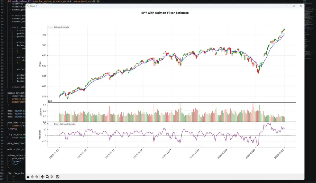
This chart shows the two main ways traders might read a Kalman filter output. Through the steady advance on the left and middle of the chart, the blue estimate rises with price but smooths out some of the smaller candle-to-candle noise. During the pullback around late March, price drops below the estimate and the residual turns negative, showing that price has moved below the model’s smoother trend estimate.

The rebound that follows is also useful. Price moves back above the Kalman estimate, the estimate turns higher, and the residual becomes strongly positive as price stretches above the filtered line. That could support a momentum reading, but it could also warn a mean-reversion trader that price has moved far from the estimate. The filter gives structure; it does not decide which interpretation is correct without the rest of the trade plan.

Kalman Filter vs Moving Averages, Regression, EMA and ADX

A Kalman filter is often compared with moving averages because both can produce a smoother line on a price chart. The logic behind them is different.

A moving average smooths price by applying a fixed averaging rule. An EMA gives more weight to recent prices, but it is still a predefined smoothing formula. A Kalman filter updates a model estimate as new observations arrive and adjusts that estimate according to the assumed noise in the data.

That makes the Kalman filter more flexible, but also easier to misuse. A moving average is simple and transparent. A Kalman filter depends more heavily on model assumptions and noise settings.

I would usually compare a Kalman estimate against a simple moving average or EMA before trusting it. If the Kalman line is only producing a more complicated version of the same signal, the extra complexity may not be worth it.

The residual is one area where the Kalman filter can become more useful. The residual is the gap between price and the Kalman estimate. Trend-following traders may care more about the direction of the estimate. Mean-reversion traders may care more about the size and behaviour of the residual.

ADX can also be useful alongside a Kalman filter. If the Kalman estimate is rising and ADX is also showing stronger trend conditions, a trend-following setup may have a better backdrop. If the Kalman residual is stretched but ADX is strong, a mean-reversion trade may be more dangerous because the market may be trending rather than rotating.

The practical test is simple. A Kalman filter should make the trading decision clearer, not merely make the chart look more advanced. If a simple EMA gives the same signal with less complexity, the simpler tool may be enough. If the Kalman estimate or residual gives a better way to define trend, spread, or mean reversion, then the extra modelling work may be justified.

Frequently Asked Questions about Kalman Filter Trading

Q: What is a Kalman filter in trading?

A Kalman filter is a model-based estimation tool. In trading, it is often used to smooth noisy price data, estimate an underlying trend, track a spread, or update a hedge ratio as new observations arrive.

Q: Does a Kalman filter predict stock prices?

It can be used in prediction models, but it does not predict prices by magic. A Kalman filter produces estimates based on a state-space model and noise assumptions. Some research has tested Kalman filters for short-term stock-price prediction, but the results depend heavily on the model, data and market conditions.

Q: Is the Kalman filter line the true value of a stock?

No. The Kalman estimate is a model output, not the market’s true value. It may be useful as a smoothed trend estimate or fair-value proxy inside a specific model, but it should not be treated as an objective valuation.

Q: How is a Kalman filter different from a moving average?

A moving average applies a fixed smoothing rule. A Kalman filter updates a model estimate as new observations arrive and adjusts that estimate based on assumed process noise and measurement noise.

Q: What is NoiseCovRatio?

NoiseCovRatio compares measurement noise with process noise. A higher ratio usually makes the filter smoother and slower. A lower ratio usually makes it more reactive but noisier.

Q: Can a Kalman filter be used for mean reversion?

Yes. Some traders use the distance between price and the Kalman estimate as a mean-reversion input. That works best when the market or spread tends to rotate around the estimate. In a strong trend, price can stay away from the estimate for a long time.

Q: Can a Kalman filter be used for trend following?

Yes. Trend-following traders may watch whether price is above a rising Kalman estimate or below a falling estimate. The signal still needs confirmation from price structure, volatility, and risk control.

Q: Can a Kalman filter be used in pairs trading?

Yes. Kalman filters are often used to estimate a dynamic hedge ratio between two instruments. That can be useful when the relationship between the pair changes over time.

Q: What is the main risk of using a Kalman filter?

The main risk is false confidence. A smooth model output can look precise, but it still depends on assumptions. If the market regime changes, the filter can become misleading.

Q: Should beginners use Kalman filters?

Beginners can learn from them, but they should not treat them as a plug-and-play trading system. It is worth comparing any Kalman estimate against simpler tools such as moving averages and testing whether the extra complexity improves the decision.

Final Thoughts

A Kalman filter can be a useful way to organise noisy market data.

It is more flexible than a simple moving average because it updates a model estimate as new observations arrive. That makes it interesting for trend smoothing, mean reversion, pairs trading, hedge-ratio estimation, and short-horizon prediction tests.

The important word is model. The Kalman line is not the market’s true value. It is an estimate created from assumptions about how the hidden state moves and how noisy the observations are.

That is why the noise settings matter. A smoother filter can make the chart easier to read, but it can react late. A faster filter can catch turns earlier, but it can also chase noise.

I would treat Kalman filter trading as a modelling problem, not an indicator shortcut. The filter can help define a trend estimate, residual, spread or hedge ratio, but the trade still needs price structure, risk control, and proper testing.

Further Reading

Related AlphaSquawk guides:

Moving Averages, for a simpler trend-smoothing baseline and Exponential Moving Average, for a faster moving-average comparison.

ADX, for judging whether a market has enough trend strength to support directional trades.

Bollinger Bands, for comparing price against volatility bands.

Other topics to explore:

Linear Regression and R-Squared, for another way to estimate trend fit and trend structure.

Pairs Trading, if you want to connect Kalman filtering to dynamic hedge ratios and spreads.

Books and references:

“A New Approach to Linear Filtering and Prediction Problems“, Rudolf E. Kálmán, 1960.

“Optimal Filtering“, Brian D. O. Anderson and John B. Moore.

“Stock Price Prediction Using Kalman Filter“, Nicholas Assimakis, Maria Adam and Dimitris Katsianis, 2025 – which tested several Kalman-filter variants for daily stock-price prediction. It reported some useful short-term prediction results, including cases where percent mean absolute error was below 2%. I would treat that as evidence that Kalman filters can be tested for prediction under specific assumptions, not as proof of a universal stock-prediction edge.

“Kalman Filter Made Easy: A Beginners Guide to the Kalman Filter and Extended Kalman Filter with Real Life Examples Supported by Python Source Code” William Franklin (2022)

“Application of Kalman Filter in the Prediction of Stock Price” by Xu Yan, Zhang Guosheng (2015) This short paper presents a real-world application of the Kalman Filter in predicting stock prices. Available at: https://www.atlantis-press.com/proceedings/kam-15/25464

“Kalman Filtering: Theory and Practice Using MATLAB” by Mohinder S. Grewal and Angus P. Andrews. (2014)