Updated May 2026: This ADL guide has been refreshed with clearer formula explanations, practical divergence warnings, Python code tweaks, and a more useful discussion of the indicator’s limitations.

Learn about the Accumulation Distribution Line technical analysis indicator, its origins, mathematical construction, and how to use it for trading. In this post, I’ve also incorporated a step-by-step Python tutorial that guides you on how to code the indicator and plot your own chart with it on for any ticker, using freely available data and software.
Introduction
The Accumulation Distribution Line, often shortened to ADL or A/D Line, is a volume-based technical indicator developed by Marc Chaikin. It tries to show whether volume is flowing into or out of a security by looking at where each candle closes within its high-low range.
The idea is straightforward. If a stock closes near the top of its daily range on high volume, ADL treats that as accumulation. If it closes near the bottom of its range on high volume, ADL treats that as distribution.
Traders mainly use ADL in two ways: to confirm the existing trend, or to spot divergence. If price is making new highs but ADL is failing to confirm, that can warn that buying pressure may be weakening. If price is making new lows but ADL is rising, that can suggest selling pressure may be fading.
This guide explains how the Accumulation Distribution Line is calculated, how to interpret ADL divergence, where the indicator can mislead you, and how to code and plot it in Python.
Key Takeaways
- The Accumulation Distribution Line (ADL) is a volume-based indicator developed by Marc Chaikin to estimate cumulative buying and selling pressure using close location and volume.
- The ADL is calculated using a three-step process involving the Money Flow Multiplier, the Money Flow Volume, and the Accumulation Distribution Line itself.
- The ADL can be used to confirm the underlying trend of a security or to anticipate reversals when the indicator diverges from the security price.
- Divergences between ADL and price can act as warning signs. A bullish divergence may suggest selling pressure is fading, while a bearish divergence may suggest buying pressure is weakening, but neither should be treated as a standalone trade signal.
- The ADL has its pros and cons. Its strength lies in its ability to consider both price and volume, providing a comprehensive view of a security’s performance. However, it can sometimes give false signals because it doesn’t consider price changes from one period to the next.
- A step-by-step Python tutorial is provided to code the ADL using the pandas library. This includes fetching financial data, calculating the ADL, and plotting it on a chart.
- ADL, like all indicators, has its limitations and should be used in conjunction with other tools and aspects of technical analysis.
- Trading involves risk, and it’s important to make informed decisions and consider multiple sources of information.
Origins of the Accumulation Distribution Line
The Accumulation Distribution Line was developed by Marc Chaikin, a stock market analyst known for developing several technical indicators. Chaikin originally referred to the ADL as the Cumulative Money Flow Line. The ADL is a running total of each period’s Money Flow Volume, which is calculated based on the relationship of the close to the high-low range and the period’s volume.
Accumulation Distribution Line Formula
The Accumulation Distribution Line is calculated in three steps.
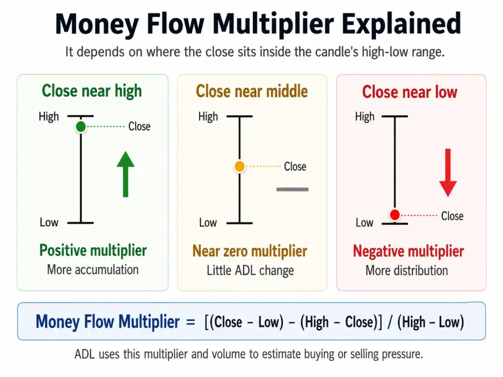
First, calculate the Money Flow Multiplier:
MFM_t = \frac{(Close_t - Low_t) - (High_t - Close_t)}{High_t - Low_t}Money Flow Multiplier at bar t = [(Closeₜ – Lowₜ) – (Highₜ – Closeₜ)] / (Highₜ – Lowₜ)
The same multiplier can also be written as:
MFM_t = \frac{(2 \times Close_t) - High_t - Low_t}{High_t - Low_t}This is the same as: Money Flow Multiplier = [(2 × Closeₜ) – Highₜ – Lowₜ] / (Highₜ – Lowₜ)
Here, t represents the current bar. The Money Flow Multiplier measures where the close sits inside that bar’s high-low range. If the close is near the high, the multiplier is positive. If the close is near the low, the multiplier is negative. If the close is near the middle, the multiplier is close to zero.
Second, multiply the Money Flow Multiplier by volume:
MFV_t = MFM_t \times Volume_t
Money Flow Volume at bar t = Money Flow Multiplierₜ × Volumeₜ
Money Flow Volume weights the multiplier by volume. A high-volume candle that closes near its high adds more positive money-flow volume. A high-volume candle that closes near its low adds more negative money-flow volume.
Third, add the current Money Flow Volume to the previous ADL value:
ADL_t = ADL_{t-1} + MFV_tADLₜ = previous ADL value + current Money Flow Volume
ADLₜ is the current Accumulation Distribution Line value. ADLₜ₋₁ is the previous value. The line is cumulative, so each new Money Flow Volume value is added to the running total.
The absolute ADL number is usually less important than the direction of the line. Traders mainly watch whether ADL is rising, falling, confirming price, or diverging from price.
Some charting platforms and data vendors use different “Accumulation/Distribution” formulas. In this section, we are using the common Chaikin-style Accumulation Distribution Line formula based on the Money Flow Multiplier and volume.
What the Money Flow Multiplier Means
The primary purpose of the Accumulation Distribution Line (ADL) is to estimate cumulative buying and selling pressure. It does this by combining volume with where each candle closes inside its high-low range. The ADL is based on the premise that if a security closes near its high for the day, then there was more buying pressure, or accumulation. Conversely, if it closes near its low, then there was more selling pressure, or distribution.
The ADL is a cumulative indicator, meaning it adds up the Money Flow Volume for each period. When the ADL is rising, it indicates that buying pressure is prevailing. When it’s falling, it indicates that selling pressure is prevailing. Traders can use the ADL to confirm the underlying trend of a security or to spot potential reversals when the ADL diverges from the price.
How Traders Use the Accumulation Distribution Line
The ADL is usually not used as a simple buy or sell trigger. It is more useful as a confirmation or warning indicator.
Trend confirmation
If price is rising and ADL is also rising, the move is being supported by volume closing toward the upper part of the range. That can confirm the strength of the trend.
If price is falling and ADL is also falling, the decline is being supported by volume closing toward the lower part of the range. That can confirm distribution.
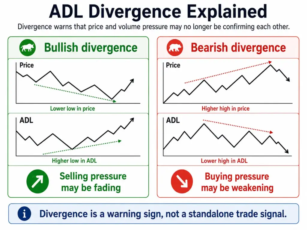
Bullish divergence
A bullish divergence occurs when price makes a lower low, but ADL makes a higher low. This suggests selling pressure may be weakening, even though the price chart still looks poor.
That does not mean the stock must reverse immediately. It is a warning to look more closely.
Bearish divergence
A bearish divergence occurs when price makes a higher high, but ADL fails to make a higher high. This suggests price may be rising without the same volume support.
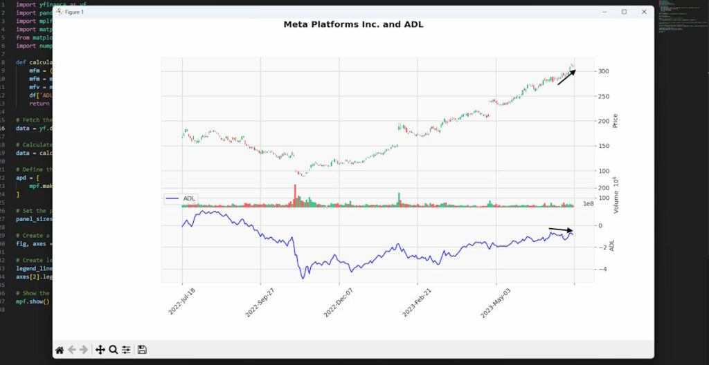
This is what makes the META example later in the article interesting. Price was pushing higher, but ADL was not confirming with the same strength. That does not guarantee a top, but it is exactly the kind of behaviour ADL is designed to highlight.
ADL vs OBV: What Is the Difference?
The Accumulation Distribution Line is often compared with On-Balance Volume, or OBV, because both use volume to judge buying and selling pressure.
The difference is how they treat price.
OBV looks at whether today’s close is higher or lower than the previous close. If the close is higher, volume is added. If the close is lower, volume is subtracted.
ADL looks inside the current candle. It asks whether the close finished near the high or near the low of that period, then weights that by volume.
That means ADL can behave differently from OBV. A stock might close higher than yesterday, causing OBV to rise, but close near the low of today’s range, which could make ADL weak. The reverse can also happen.
Neither indicator is automatically better. ADL is useful when you care about where price closed within the day’s range. OBV is simpler and focuses on whether price closed up or down compared with the previous period.
Pros and Cons of the Accumulation Distribution Line
The main advantage of ADL is that it combines price location and volume. It can help traders see whether a trend is being confirmed by volume pressure, and it can highlight divergences that may not be obvious from price alone.
It is also simple to calculate and easy to plot, which makes it useful for screeners, chart studies and Python-based research.
But ADL has important weaknesses.
The biggest limitation is that it does not directly account for the change from one candle’s close to the next. It only looks at where the close sits inside the current candle’s high-low range.
That can create odd signals. For example, a stock could gap down sharply, recover during the session, and close near the high of the day. ADL may rise because the close was strong relative to that day’s range, even though the stock is still lower than the previous close.
ADL can also be distorted by unusual volume, earnings gaps, news shocks, index rebalancing, or low-liquidity periods. For that reason, divergence should be treated as a warning, not as a standalone trade signal.
The best use of ADL is alongside price structure, trend, support and resistance, volume context, and other tools such as RSI, MACD, moving averages or fundamental catalysts.
Coding the Accumulation Distribution Line
For those interested in algorithmic trading, it can be useful to know how to code the Accumulation Distribution Line in popular trading languages. In this section, we’ll provide an example in Python using the pandas library, which is widely used for data analysis in finance.
import pandas as pd
import numpy as np

def calculate_adl(df):
    # Calculate the Money Flow Multiplier
    mfm = ((df['Close'] - df['Low']) - (df['High'] - df['Close'])) / (df['High'] - df['Low'])
    mfm = mfm.replace([np.inf, -np.inf], 0).fillna(0)

    # Calculate the Money Flow Volume
    mfv = mfm * df['Volume']

    # Calculate the Accumulation Distribution Line
    df['ADL'] = mfv.cumsum()

    return df

# Assume df is a DataFrame with 'High', 'Low', 'Close', and 'Volume' columns
df = calculate_adl(df)Build ADL with Python and Plot it on a Chart
Let’s assume you want to use the above code with some downloaded data for a stock and plot that data with the ADL indicator on it. You could do this by using the free VSCode software from Microsoft and once Python (also free) is installed you can then follow my steps below.
Before proceeding, please ensure that you have the necessary Python packages installed. You can do so by running the following commands in the terminal:
pip install pandas
pip install numpy
pip install yfinance
pip install matplotlib
pip install mplfinanceNow create a new Python file called something like ADL.py and start to add the below code blocks into it in the same order:
Step 1: Import necessary libraries
import yfinance as yf
import pandas as pd
import numpy as np
import mplfinance as mpf
import matplotlib.pyplot as plt
from matplotlib.lines import Line2DIn this step, we’re importing all the necessary libraries.
pandasis a data manipulation library.numpyis used for numerical operations. In this example, we use it to handle infinite values that can appear if a candle’s high and low are the same.yfinanceis used to fetch financial data.mplfinanceis a library specifically designed for financial data visualisation.matplotlibis a plotting library, andLine2Dis a class for creating line segments, which we will use to create the legend for our plot.
Step 2: Define the ADL calculation function
def calculate_adl(df):
    mfm = ((df['Close'] - df['Low']) - (df['High'] - df['Close'])) / (df['High'] - df['Low'])
    mfm = mfm.replace([np.inf, -np.inf], 0).fillna(0)
    mfv = mfm * df['Volume']
    df['ADL'] = mfv.cumsum()
return dfHere, we define a function to calculate the Accumulation/Distribution Line (ADL). The function takes a dataframe with High, Low, Close and Volume columns, calculates the Money Flow Multiplier and Money Flow Volume, then cumulatively sums the Money Flow Volume to create the ADL. The replace and fillna step handles cases where the high and low are the same, which would otherwise create infinite or missing values.
Step 3: Fetch the data
data = yf.download('META', start='2022-07-17', end='2023-07-17')
This step uses yfinance to download historical price data for Meta Platforms Inc. (formerly Facebook, ticker symbol: META) for the period from July 1, 2022, to July 1, 2023. The fetched data includes ‘Open’, ‘High’, ‘Low’, ‘Close’, ‘Adj Close’, and ‘Volume’ information.
Step 4: Calculate the ADL
data = calculate_adl(data)We call the calculate_adl() function on our data to calculate the ADL and add it as a new column to the dataframe.
Step 5: Define the additional plots
apd = [
    mpf.make_addplot(data['ADL'], panel=2, color='b', secondary_y=False, ylabel='ADL')
]This step sets up the additional plot for the ADL. We use mpf.make_addplot() to create this additional plot, specifying that it should be drawn on the third panel (panel indices start at 0), with blue color, and with the y-axis label ‘ADL’.
Step 6: Set the panel sizes and create the subplot
panel_sizes = (5, 1, 3)
fig, axes = mpf.plot(data, type='candle', style='yahoo', addplot=apd, volume=True, panel_ratios=panel_sizes, title='Meta Platforms Inc. and ADL', returnfig=True)We specify the sizes of the panels and then create the plot using mpf.plot(). The parameters used here configure the plot to use candlestick charts, the ‘yahoo’ style, include volume, and have a title.
Step 7: Create the legend
legend_lines = [Line2D([0], [0], color='b', lw=1.5)]
axes[2].legend(legend_lines, ['ADL'], loc='lower left')We create a legend for the ADL plot using a dummy line from matplotlib.lines.Line2D.
Step 8: Show the plot
mpf.show()Finally, we use mpf.show() to display the plot.
META Example: ADL Bearish Divergence
When you run the script, it should download the data, calculate the ADL, and display a plot with the price data and ADL indicator looking like mine below:
Conclusion
In conclusion, the Accumulation Distribution Line is a powerful tool that can help traders gauge the cumulative flow of money into and out of a security. By taking into account both price and volume, the ADL provides a more comprehensive view of a security’s performance than price alone. However, like all indicators, it has its limitations and should be used in conjunction with other tools and aspects of technical analysis.
Whether you’re confirming the underlying trend of a security, spotting potential reversals, or coding your own trading algorithm, understanding the ADL can give you an edge in the market. As always, remember that trading involves risk, and it’s important to make informed decisions and consider multiple sources of information.
Bibliography
- Morris, G. L. (2005). The Complete Guide to Market Breadth Indicators: How to Analyze and Evaluate Market Direction and Strength. McGraw-Hill.
- Murphy, John J. (1999). Technical Analysis of the Financial Markets. New York Institute of Finance.
- Pring, M. J. (2014). Technical Analysis Explained: The Successful Investor’s Guide to Spotting Investment Trends and Turning Points. 5th Edition. McGraw-Hill.