Updated May 2026: I’ve refreshed this ATR guide with clearer true range formulas, more practical notes on stop placement and position sizing, and an updated Python walkthrough.
What Is the Average True Range Indicator?
Average True Range, usually shortened to ATR, is a volatility indicator.
It measures how much a market has been moving over a chosen number of bars. A high ATR means the market has been making larger moves. A low ATR means the market has been quieter.
ATR does not tell you direction. A rising ATR can appear during a rally, a sell-off, or a chaotic two-way market. It only tells you that the size of the price movement has increased.
That makes ATR useful for risk management. Traders often use it to think about stop distance, position size, volatility filters, and whether a market is too quiet or too active for a particular strategy.
For example, a stop that makes sense when ATR is small may be far too tight when ATR is large. The same two-point stop can mean very different things on two different markets or even on the same market in two different volatility regimes.
In this guide I’ll walk through the true range formula, how Wilder’s ATR smoothing works, how ATR% helps compare different markets, and how to calculate and plot ATR in Python.
How Average True Range Is Calculated
ATR begins with True Range.
True Range tries to capture the full movement of the current bar, including any gap from the previous close. That is why it uses three possible distances and takes the largest one.
Before the formulas, here are the symbols:
H means the current high.
L means the current low.
Cprev means the previous close.
TR means True Range.
ATR means Average True Range.
n means the ATR period.
t means the current bar.
TR_t = \max \left( H_t - L_t,\ |H_t - C_{t-1}|,\ |L_t - C_{t-1}| \right)True Range = the largest of current high – current low, current high – previous close, or current low – previous close
The first part, high minus low, measures the current bar’s normal range.
The second and third parts capture gaps from the previous close. This is why True Range can be larger than the simple high-low range. If a market gaps up or gaps down, ATR is designed to notice that movement.
Wilder ATR smoothing
Once True Range has been calculated, ATR smooths it over time. Wilder’s common method is a recursive smoothing formula.
ATR_t = \left(\frac{(n - 1) \times ATR_{t-1} + TR_t}{n}\right)ATR of current bar = ((n – 1) × previous ATR + current True Range) / n
This is similar in spirit to an exponential smoothing method, but Wilder’s version uses 1 / n as the smoothing factor.
A 14-period ATR is common. On a daily chart, that means 14 daily bars. On a 5-minute chart, it means 14 five-minute bars. The logic is the same, but the trading use is very different.
Average True Range Percent (ATR%)
ATR is an absolute number. If a stock has an ATR of 5, that means it has recently been moving about 5 price units per bar, depending on the timeframe used.
That is useful on one chart, but harder to compare across markets. A 5-point ATR means something very different on a $20 stock and a $500 stock.
ATR% solves that by expressing ATR as a percentage of price.
ATR\% = \frac{ATR}{Close} \times 100ATR% = ATR / current close × 100
ATR% makes volatility easier to compare across different markets and price levels. It is especially useful when scanning a list of instruments or comparing a high-priced stock with a lower-priced one.
How Traders Use ATR
ATR is mainly a volatility tool. It tells you how much the market has been moving, not which direction it is likely to move next.
That sounds simple, but it is useful. A market with a high ATR needs different risk handling from a market with a low ATR. The same stop size, position size or target can make sense in one volatility regime and be completely wrong in another.
I use ATR as a way to ask: how much room does this market normally need to move?
That question can help with stops, position sizing, breakout filters, volatility comparisons and avoiding trades when the market is too quiet or too jumpy.
ATR for stop placement
One common ATR use is stop placement.
If a market normally moves around 2 points per bar, a 0.5-point stop may be too tight. If a market normally moves 0.2 points per bar, a 2-point stop may be too wide for the trade being attempted.
A common method is to place a stop a multiple of ATR away from the entry. For example, a trader might use 1.5 × ATR or 2 × ATR as a rough volatility-adjusted stop distance.
This does not mean ATR magically finds the correct stop. It only gives a volatility reference. Price structure still matters. A stop placed at 2 × ATR but sitting in the middle of obvious support or resistance may still be badly placed.
ATR for position sizing
ATR can also help with position sizing.
A higher ATR means the market is moving more. If you trade the same number of contracts or shares during a high-ATR period, the money risk can be much larger than during a quiet period.
For example, if one market has an ATR of 1 and another has an ATR of 5, the second market is moving roughly five times as much in price terms. If the position size is not adjusted, the risk may be very different even if the trade setup looks similar.
This is why some traders reduce position size when ATR rises and increase it only when the volatility risk is lower. The goal is not to avoid volatility completely. It is to stop volatility from deciding the size of the loss for you.
ATR for breakouts and quiet markets
ATR can also help identify changing volatility conditions.
A low ATR means the market has been quiet. That can happen before a breakout, but low ATR alone does not tell you which way price will move.
A rising ATR after a breakout can suggest the market is expanding into a more active phase. That can support a breakout view if price structure agrees.
The mistake is assuming that low ATR always means a big move is coming. Sometimes a quiet market stays quiet.
ATR before major events
ATR is less helpful when the next big move is likely to come from a scheduled event.
For example, before earnings, a central-bank decision or a major economic release, the recent trading range may shrink while traders wait. ATR may fall, making the market look quieter than it really is.
That can make ATR-based stops look too tight just before the event that blows the range open.
This is where the wider calendar matters. ATR measures recent movement. It does not know that non-farm payrolls, an interest-rate decision or an earnings release is coming.
How to Interpret ATR
A rising ATR means recent price ranges are getting larger.
A falling ATR means recent price ranges are getting smaller.
That is all ATR says. It does not tell you whether the next move should be up or down.
| ATR reading | What it shows | How I would read it |
|---|---|---|
| ATR rising | Price ranges are expanding | Volatility is increasing |
| ATR falling | Price ranges are contracting | Volatility is decreasing |
| High ATR after breakout | Larger ranges after a break | Breakout may have energy |
| Low ATR before a break | Quiet market conditions | Possible compression, but no direction |
| High ATR into event risk | Recent or expected volatility | Stops and size need care |
| ATR spike | Sudden range expansion | Check news, gaps or one-off event |
ATR vs Bollinger Bands
ATR and Bollinger Bands are both used in volatility analysis, but they measure volatility differently.
ATR measures trading range. It looks at high, low and previous close to capture the size of recent price movement, including gaps.
Bollinger Bands use standard deviation around a moving average. They measure how dispersed price is around its average.
That means ATR is often more directly useful for stop placement and position sizing. Bollinger Bands are often used to study price stretching away from its average, squeeze setups and mean-reversion conditions.
Neither of them is automatically better. They answer different volatility questions.
| Tool | Volatility input | Common use | Main warning |
|---|---|---|---|
| ATR | True Range | Stops, position sizing, volatility filters | No direction signal |
| ATR% | ATR divided by price | Compare volatility across markets | Still backward-looking |
| Bollinger Bands | Standard deviation | Squeeze, stretched price, mean reversion | Price can ride the band in trends |
| Keltner Channels | ATR around a moving average | Trend, breakout and pullback context | Breakouts can fail |
ATR is also part of many volatility-channel tools. For example, Keltner Channels usually place bands a multiple of ATR above and below a moving average. Bollinger Bands, by contrast, use standard deviation around a moving average.
ATR Pros and Cons
ATR is useful because it gives traders a practical volatility number. It turns recent price movement into something that can be used for stop distance, position sizing and volatility comparison.
Its biggest strength is also its limit. ATR is based on past price ranges. It adapts to volatility after it appears; it does not know what the next candle will do.
| Strength | Why it helps |
|---|---|
| Measures volatility directly | Shows how much the market has been moving |
| Includes gaps | True Range captures movement from the previous close |
| Useful for stops | Helps avoid using fixed stops in changing volatility |
| Useful for position sizing | Helps scale risk when markets move more or less |
| Works across timeframes | Can be used on daily, intraday or weekly charts |
| Weakness | Why it matters |
|---|---|
| No direction signal | ATR does not say whether price should rise or fall |
| Backward-looking | It reflects recent volatility, not future volatility |
| Can be too low before events | Quiet pre-event trading can understate upcoming risk |
| Can spike after the damage | ATR may rise after a sharp move has already happened |
| Needs price context | Stop placement still needs support, resistance and structure |
Quick ATR Takeaways Before We Code
- ATR stands for Average True Range.
- ATR measures volatility, not direction.
- True Range uses the largest of high-low, high-previous close, or low-previous close.
- ATR smooths True Range over a chosen number of bars.
- A rising ATR means recent ranges are expanding.
- A falling ATR means recent ranges are contracting.
- ATR can help with stop placement and position sizing.
- ATR% makes volatility easier to compare across different price levels.
- ATR can be misleading before major scheduled events because recent ranges may be quiet before the move.
- The Python tutorial below calculates True Range, ATR and ATR%, then plots ATR below a candlestick chart.
Now we can build ATR ourselves. The Python section below calculates True Range, applies Wilder-style ATR smoothing, adds ATR%, and plots the result under a price chart.
Coding ATR in Python and Plotting the Chart
Now we can build ATR in Python.
I am going to keep this as a step-by-step tutorial rather than dropping in one large script. Each Python-labelled block goes into the same file, in order. By the end, we will have downloaded market data, calculated True Range, ATR and ATR%, and plotted them below a candlestick chart.
For this example I use META, as in the earlier version of this article, but with a more recent date range.
Step 1: Install the Python libraries
This guide assumes you already have Python installed and are using Visual Studio Code.
Open a terminal in VS Code by clicking Terminal > New Terminal, then run:
python -m pip install yfinance pandas mplfinance matplotlibOn some Windows machines, this version works instead:
py -m pip install yfinance pandas mplfinance matplotlibStep 2: Create the file and import the libraries
Create a new Python file and save it as:
atr_indicator.py
At the top of the file, add:
import pandas as pd
import yfinance as yf
import mplfinance as mpf
from matplotlib.lines import Line2D
pandas stores the market data in a table and handles the calculations.
yfinance downloads the price data.
mplfinance draws the candlestick chart.
Line2D lets us create a clean legend for the ATR and ATR% lines.
Step 3: Add the settings
Next, add the settings near the top of the file.
ticker = "META"
chart_title = "Meta Platforms"

start_date = "2025-05-01"
end_date = "2026-05-01"

atr_period = 14
ticker is the Yahoo Finance symbol.
chart_title is the title printed on the chart.
The dates use YYYY-MM-DD format. yfinance treats the end date as a cut-off, so you can push it one trading day later if you want the most recent available bar included.
atr_period controls how many bars are used in the ATR smoothing calculation.
Step 4: Download the market data
Now download the market data.
data = yf.download(
    ticker,
    start=start_date,
    end=end_date,
    auto_adjust=True,
    progress=False,
    multi_level_index=False
)

if data.empty:
    raise RuntimeError("No data was downloaded. Check the ticker symbol and date range.")

if isinstance(data.columns, pd.MultiIndex):
    data.columns = data.columns.get_level_values(0)

data.index = pd.DatetimeIndex(data.index)This downloads open, high, low, close and volume data.
auto_adjust=True keeps the price series adjusted where applicable.
progress=False removes the download progress bar.
multi_level_index=False keeps the columns easier to work with.
The final line makes sure the index is treated as dates, which mplfinance expects when plotting.
Step 5: Define the True Range and ATR functions
Now define the functions that calculate True Range, ATR and ATR%.
def calculate_true_range(data):
    high = data["High"]
    low = data["Low"]
    close = data["Close"]

    high_low = high - low
    high_prev_close = (high - close.shift(1)).abs()
    low_prev_close = (low - close.shift(1)).abs()

    true_range = pd.concat(
        [high_low, high_prev_close, low_prev_close],
        axis=1
    ).max(axis=1)

    return true_range


def calculate_atr(data, period=14):
    true_range = calculate_true_range(data)

    atr = pd.Series(index=true_range.index, dtype="float64")

    # First ATR value: simple average of the first period of True Range values
    atr.iloc[period - 1] = true_range.iloc[:period].mean()

    # Wilder-style smoothing
    for i in range(period, len(true_range)):
        atr.iloc[i] = ((period - 1) * atr.iloc[i - 1] + true_range.iloc[i]) / period

    return atr


def calculate_atr_percent(data, atr):
return (atr / data["Close"]) * 100calculate_true_range() works out the largest of the three True Range components.
calculate_atr() applies Wilder-style smoothing to True Range.
calculate_atr_percent() converts ATR into a percentage of the closing price, which makes it easier to compare volatility across different price levels.
Step 6: Calculate ATR and ATR%
Now call the functions and add the results to the data table.
data["True Range"] = calculate_true_range(data)
data["ATR"] = calculate_atr(data, period=atr_period)
data["ATR%"] = calculate_atr_percent(data, data["ATR"])

plot_data = data.dropna(subset=["ATR", "ATR%"])Think of data as a spreadsheet. It already has Open, High, Low, Close and Volume columns. This step adds True Range, ATR and ATR%.
dropna() removes the early blank rows before plotting. Those blanks appear because the ATR calculation needs enough bars before it can produce values.
Step 7: Define the ATR chart lines
Next we tell mplfinance how to draw ATR and ATR% below the price chart.
atr_plots = [
    mpf.make_addplot(
        plot_data["ATR"],
        panel=2,
        color="green",
        width=1.2,
        ylabel="ATR"
    ),
    mpf.make_addplot(
        plot_data["ATR%"],
        panel=3,
        color="red",
        width=1.0,
        ylabel="ATR%"
    )
]The green line is ATR.
The red line is ATR%.
They are plotted in separate panels because ATR is measured in price units, while ATR% is measured as a percentage of price.
Step 8: Create the chart
Now create the candlestick chart.
fig, axes = mpf.plot(
    plot_data,
    type="candle",
    style="yahoo",
    volume=True,
    addplot=atr_plots,
    panel_ratios=(3, 1, 1.2, 1.2),
    title=f"{chart_title} with ATR ({atr_period}) and ATR%",
    figsize=(11, 8),
    returnfig=True
)

fig.subplots_adjust(
    left=0.07,
    right=0.90,
    top=0.92,
    bottom=0.16,
    hspace=0.05
)type="candle" gives us the candlestick chart.
volume=True adds the volume panel.
addplot=atr_plots adds the ATR and ATR% lines.
panel_ratios controls the relative size of the price, volume, ATR and ATR% panels.
subplots_adjust gives the chart extra room so the right-hand labels and angled dates are not clipped.
Step 9: Add the legend and show the chart
Finally, add a legend, save the image and show the chart.
legend_items = [
    Line2D([], [], color="green", label="ATR"),
    Line2D([], [], color="red", label="ATR%")
]

fig.legend(
    handles=legend_items,
    loc="center left",
    bbox_to_anchor=(0.04, 0.5),
    frameon=False
)

fig.savefig("atr_indicator_chart.png", dpi=150, bbox_inches="tight")

mpf.show()fig.legend() adds a chart legend.
fig.savefig() saves the chart as a PNG image in the same folder as the script.
mpf.show() opens the chart window.
Step 10: Run the script
Save atr_indicator.py by pressing Ctrl+S.
The easiest route is usually to click the play button in the top-right corner of VS Code. If that works, the chart window should open.
You can also run it from the terminal. Open Terminal > New Terminal, move into the folder where you saved the script, then run:
python atr_indicator.pyOn some Windows setups, use:
py atr_indicator.pyYour chart should show Meta candlesticks, volume, ATR and ATR% in separate panels.
You can double check it with something like Yahoo Finance charts using their 14 period ATR with the same dates and you’ll see our green line is identical, which is always reassuring.
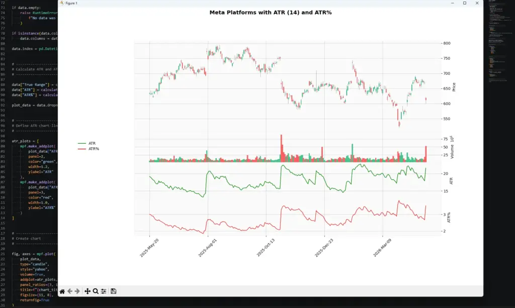
The ATR% shown in the first chart is calculated as ATR divided by the current closing price. This makes the volatility reading easier to compare across different markets and price levels. A $10 ATR means something very different on a $100 stock than on a $1,000 stock, but ATR% puts both into percentage terms.
A Different True Range Percent Approach
The ATR% in the first chart is calculated as:
ATR\% = \frac{ATR}{Close} \times 100ATR% = ATR / current close × 100
That version is useful because it expresses volatility as a percentage of the current price. It lets you compare ATR across different markets and price levels.
There is another useful calculation, but I would not call it ATR%. I would call it Current True Range as a percentage of ATR.
This asks a different question:
How large was the latest bar’s true range compared with the recent average true range?
If the value is near 100%, the latest true range is close to normal for the lookback period. If it is near 200%, the latest true range is roughly twice the recent ATR. If it is several hundred percent, the market may have gapped or produced an unusually large bar.
This can be useful when you want to spot unusually large candles, earnings gaps, shock moves, or sudden volatility breaks.
TR\%ATR_t = \frac{TR_t}{ATR_t} \times 100Current True Range % of ATR = current true range / ATR × 100
In Python, if we already have a calculate_true_range() function and an ATR column, the calculation is simple:
def calculate_true_range_percent_of_atr(data, atr):
    true_range = calculate_true_range(data)
return (true_range / atr) * 100Then add the new column like this:
data["TR % of ATR"] = calculate_true_range_percent_of_atr(data, data["ATR"])Use the two percent calculations for different jobs:
| Calculation | Formula | What it tells you |
|---|---|---|
| ATR% of price | ATR / Close × 100 | Shows ATR as a percentage of price, useful for comparing volatility across markets |
| Current True Range % of ATR | Current True Range / ATR × 100 | Shows whether the latest bar is unusually large compared with recent volatility |
So after plugging that into our code, the red line in the chart now shows the current bar’s True Range as a percentage of recent ATR:
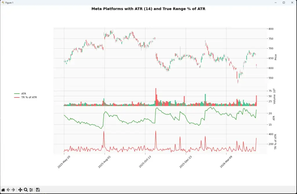
This second chart uses a different calculation from normal ATR%. Instead of dividing ATR by the current closing price, it compares the current bar’s True Range with the recent ATR.
That makes the red line a “range shock” measure. A value around 100% means the latest bar is close to normal for the lookback period. A value around 200% means the bar is roughly twice the recent ATR. Large spikes can appear around earnings gaps, surprise news, macro events or other sudden volatility breaks.
Practical ATR Examples
A few examples make ATR easier to understand.
Example 1: Stop distance
Suppose a stock is trading around $100 and its 14-period ATR is 2. That tells us the stock has recently been moving about $2 per bar on average.
A stop 20 cents away would probably be too tight for most swing setups, because normal movement could knock it out quickly. A stop based on 1.5 or 2 times ATR would give the trade more room, although the exact stop still needs to fit the chart structure.
Example 2: Position sizing
Now imagine two stocks.
Stock A has an ATR of 1.
Stock B has an ATR of 5.
If you buy the same number of shares in both, Stock B carries much more price movement risk. ATR can help you reduce size in the more volatile market so the trade risk is not wildly different.
Example 3: Event risk
ATR is based on recent price ranges. It does not know that earnings, payrolls, inflation data or a central-bank decision is coming.
If a market has been quiet before a major event, ATR may be low. That can make ATR-based stops look sensible just before volatility expands sharply. This is one reason I would never use ATR without checking the wider calendar.
Final Thoughts on ATR
ATR is useful because it gives traders a practical measure of recent volatility. It does not predict direction, but it can help with stop placement, position sizing, volatility filters and comparing different markets.
The biggest mistake is treating ATR as if it knows what will happen next. It measures recent range. It does not know about the next earnings report, central-bank decision, payrolls release or surprise headline.
I would use ATR as a risk and volatility tool first. The trade direction still needs to come from price structure, trend analysis, momentum, fundamentals, or whatever method you are actually testing.
Further Reading
Wilder, J. Welles. “New Concepts in Technical Trading Systems.” Trend Research, 1978.
For related AlphaSquawk guides, see our ATR-based Keltner Channel guide, Bollinger Bands guide, and risk-management / stop-placement articles where relevant.