Updated May 2026: This ASI guide has been refreshed with clearer formula notes, code tweaks, a better explanation of the limit move value, and a new Python chart example using recent data.

Introduction
The Accumulative Swing Index, usually shortened to ASI, is a technical indicator developed by J. Welles Wilder. It builds on Wilder’s Swing Index by comparing the current bar’s open, high, low and close with the previous bar’s prices.
Wilder’s aim was to cut through some of the noise inside ordinary bar and candlestick charts and create a line that could be used to judge the underlying direction of price swings. In that sense, ASI is not a normal oscillator like RSI, and it is not a volume indicator like OBV or the Accumulation Distribution Line. It is a price-swing indicator.
Traders mainly use ASI to confirm trend direction, compare indicator trendlines with price trendlines, and look for possible divergence or failed breakouts. It is most often discussed in a futures context, partly because the original formula includes a limit move value.
This guide explains how ASI is constructed, what the limit move value means, how traders use the indicator, and what to watch out for before coding it in Python or R.
Origins of Accumulative Swing Index (ASI)
The Accumulative Swing Index was developed by J. Welles Wilder and introduced in his 1978 book New Concepts in Technical Trading Systems. Wilder also created several other well-known indicators, including RSI, ATR and the Directional Movement system.
ASI is based on the Swing Index. The Swing Index measures each individual price swing using the relationship between the current bar and the previous bar. The Accumulative Swing Index then adds those Swing Index values together over time to form a cumulative line.
That distinction matters. The Swing Index is the one-period calculation. ASI is the running total. Traders usually study the ASI line because it can be compared with price trendlines, support and resistance, and breakout behaviour.
Mathematical Construction
The Accumulative Swing Index (ASI) is derived from the Swing Index (SI), which is calculated using a specific formula. Here’s how it works:
The Swing Index (SI) is calculated as follows:
SI = 50 \times \left[ \frac{(C_2 - C_1) + 0.5(C_2 - O_2) + 0.25(C_1 - O_1)}{R} \right] \times \frac{K}{T}which can also be written as SI = 50 × [((C₂ – C₁) + 0.5(C₂ – O₂) + 0.25(C₁ – O₁)) / R] × K / T
In this formula:
- SI represents the Swing Index for the current bar.
- C₂ is the closing price for the current bar.
- C₁ is the closing price for the previous bar.
- O₂ is the opening price for the current bar.
- O₁ is the opening price for the previous bar.
- H₂ is the highest price for the current bar.
- L₂ is the lowest price for the current bar.
- R is a variable range value based on the relationship between the current bar and the previous close.
- K is the largest absolute price difference used to scale the move.
- T is the limit move value, or price-limit value, used to scale the Swing Index.
Some formula sources use L for the limit move value, but that can be confusing because L is also commonly used for the low price. In this article, T is used for the limit move value.
K is the largest absolute value of the following two differences:
- The difference between the current bar’s high and the previous bar’s close: |H₂ – C₁|
- The difference between the current bar’s low and the previous bar’s close: |L₂ – C₁|
In plain English, K looks at how far the current bar stretched away from the previous close.
The variable R is determined by first finding the largest absolute value of the following:
- |H₂ – C₁|
- |L₂ – C₁|
- |H₂ – L₂|
The calculation for R then depends on which of those is largest:
- If |H₂ – C₁| is largest, then R = |H₂ – C₁| – 0.5 × |L₂ – C₁| + 0.25 × |C₁ – O₁|
- If |L₂ – C₁| is largest, then R = |L₂ – C₁| – 0.5 × |H₂ – C₁| + 0.25 × |C₁ – O₁|
- If |H₂ – L₂| is largest, then R = |H₂ – L₂| + 0.25 × |C₁ – O₁|
Once the Swing Index is calculated for the current bar, it is added to the previous ASI value to form the Accumulative Swing Index:
ASI = Previous ASI + Current SI
That is why ASI is a cumulative indicator. The Swing Index measures one bar’s swing movement, while ASI adds those swing values together over time. As a price-based indicator, ASI generally follows the broad direction of the price chart, but it can also diverge from price or confirm trendline breaks.
Later in this post, we will show how to code this formula in Python. The important coding point is that the limit move value must be handled deliberately. For futures, that value should ideally come from the exchange or platform specification. For stocks or ETFs, any percentage-based setting is only a proxy.
Purpose and Design
The purpose of ASI is to create a cumulative swing line that can be compared with the price chart.
Wilder described the Swing Index as an attempt to isolate the “real” price movement from the maze of open, high, low and close prices. That does not mean ASI reveals a hidden true price. It means the indicator applies a specific formula to the relationship between current and previous prices, then accumulates those values into a line.
This makes ASI most useful as a confirmation tool. If price is trending higher and ASI is also trending higher, the indicator supports the idea that the move is intact. If price breaks a trendline and ASI also breaks a comparable trendline, traders may treat that as stronger confirmation.
If price appears to break out but ASI does not confirm, the breakout may deserve more caution.
How to Use Accumulative Swing Index (ASI) for Trading
ASI is best used as a confirmation tool rather than a standalone entry system.
Trend confirmation: If price is rising and ASI is also rising, the indicator is confirming the direction of the move. If price is falling and ASI is falling, it supports the idea that the downtrend is still intact.
Breakout confirmation: One common use is to draw trendlines on both price and the ASI line. If price breaks a trendline and ASI also breaks its own comparable trendline, traders may treat that as stronger confirmation. If price breaks out but ASI does not, the move may deserve more caution.
Divergence: ASI divergence occurs when price and ASI stop agreeing. For example, price may make a new high while ASI fails to make a new high. That can suggest the move is weakening. A market can keep trending despite divergence, so this should be treated as a warning rather than an automatic trade signal.
The key point is that ASI should not be asked to make the whole trading decision. It is one layer of evidence alongside price structure, support and resistance, volume, market context and risk management. Like all technical indicators, it should be used with other tools rather than treated as a standalone signal.
Limit Move Value
The limit move value is one of the trickier parts of ASI.
In Wilder/CQG-style notation, the formula uses a one-direction limit move value to scale the Swing Index. CQG describes this as the value of a limit move in one direction and says it can be looked up using CSpec (contract specifications) or looking up the limits from an exchange’s website.
That makes sense for futures contracts where exchange-defined price limits may exist. For example, some commodity futures such as grains have rules that limit how far the contract can move in one session.
For stocks, ETFs and many other markets, there may not be an obvious daily limit move value. In that case, charting packages and custom code may use a fixed value, a percentage proxy, or another internal setting. That means two ASI charts can differ if they use different assumptions.
This is important when coding ASI yourself. If your Python version uses a percentage of the previous close as a proxy for the limit move value, say so clearly. Do not pretend it is the official Wilder value for every market.
For this article, the key rule is: use the proper exchange or platform limit move value when one exists. If you use a proxy, document it.
Pros and Cons of Using ASI
Like any technical indicator, ASI has strengths and weaknesses.
Pros:
Trend confirmation: ASI can help confirm whether price swings support the direction of the trend.
Breakout confirmation: Traders can compare trendlines on price with trendlines on the ASI line. When both break in the same direction, the breakout may carry more weight.
Price-structure focus: ASI uses the relationship between the current and previous open, high, low and close, which makes it different from simpler close-to-close indicators.
Useful for futures analysis: ASI was designed with futures-style market structure in mind, including the idea of a limit move value.
Cons:
Formula complexity: ASI is more complicated than many indicators, which makes it easier to code incorrectly or misunderstand.
Limit move assumption: The price limit value is not always obvious, especially for stocks or ETFs. Different assumptions can produce different ASI values.
False confirmation: ASI can confirm moves that still fail. It should not be used as a standalone trading system.
Lag and smoothing effect: Because ASI is cumulative, it can sometimes react after a move is already underway.
Not a volume indicator: ASI does not measure volume pressure. If you want to know whether a move is supported by volume, use a volume-based tool such as OBV or the Accumulation Distribution Line alongside it.
ASI vs Volume Indicators such as ADL and OBV
ASI is a price-based indicator. It uses open, high, low and close relationships, but it does not use volume.
That makes it different from indicators such as the Accumulation Distribution Line and On-Balance Volume, which use volume to estimate buying and selling pressure.
So if you want to study whether a price move is being supported by volume, ASI is not the right tool by itself. If you want to study whether price swings and breakouts are being confirmed by a Wilder-style swing calculation, ASI may be more relevant.
Coding ASI in Python and R
Implementing ASI means translating the Swing Index formula into code, then cumulatively summing each Swing Index value to create the Accumulative Swing Index.
The important point is the limit move value. In CQG/Wilder-style notation this is the value used to scale the Swing Index. For futures, it should ideally come from the relevant exchange specification or your charting platform’s contract specification. For stocks or ETFs, there is usually no obvious daily limit move value, so any percentage-based value is only a proxy.
The examples below use a price_limit input so the assumption is visible rather than hidden inside the formula.
Python ASI function
import numpy as np
import pandas as pd

def calculate_asi(data, price_limit):
    """
    Calculate the Accumulative Swing Index using Wilder/CQG-style logic.

    Parameters
    ----------
    data : pandas.DataFrame
        Must contain Open, High, Low and Close columns.

    price_limit : float or pandas.Series
        The one-direction limit move value used to scale the Swing Index.
        For futures, use the relevant exchange/platform value if available.
        For stocks or ETFs, a percentage proxy can be used for demonstration,
        but it should be clearly documented.
    """

    data = data.copy()

    # Previous bar values
    o1 = data["Open"].shift(1)
    c1 = data["Close"].shift(1)

    # Current bar values
    o2 = data["Open"]
    h2 = data["High"]
    l2 = data["Low"]
    c2 = data["Close"]

    # Components used to calculate K and R
    high_from_prev_close = (h2 - c1).abs()
    low_from_prev_close = (l2 - c1).abs()
    current_range = (h2 - l2).abs()

    # K is the largest absolute difference between current high/low and previous close
    k = np.maximum(high_from_prev_close, low_from_prev_close)

    # R depends on which range relationship is largest
    r = np.where(
        (high_from_prev_close >= low_from_prev_close) & (high_from_prev_close >= current_range),
        high_from_prev_close - 0.5 * low_from_prev_close + 0.25 * (c1 - o1).abs(),
        np.where(
            (low_from_prev_close >= high_from_prev_close) & (low_from_prev_close >= current_range),
            low_from_prev_close - 0.5 * high_from_prev_close + 0.25 * (c1 - o1).abs(),
            current_range + 0.25 * (c1 - o1).abs()
        )
    )

    numerator = (c2 - c1) + 0.5 * (c2 - o2) + 0.25 * (c1 - o1)

    si = 50 * (numerator / r) * (k / price_limit)
    si = pd.Series(si, index=data.index).replace([np.inf, -np.inf], 0).fillna(0)

    data["SI"] = si
    data["ASI"] = data["SI"].cumsum()

    return data
Here is what the function does:
- It shifts the open and close columns back one bar so the current bar can be compared with the previous bar.
- It calculates K from the largest absolute move between the current bar’s high or low and the previous close.
- It calculates R using the largest of three relationships: current high to previous close, current low to previous close, or the current high-low range.
- It calculates the Swing Index from the Wilder/CQG-style formula.
- It cumulatively sums the Swing Index values to create ASI.
The price_limit input is deliberate. It should not be hidden inside the function. If you are using ASI on a futures contract, use the relevant exchange or platform value where available. If you are plotting ASI on a stock or ETF, a percentage of the previous close can be used as a demonstration proxy, but it is not an official limit move value.
In R it would be:
calculate_asi <- function(data, price_limit) {

  # Previous bar values
  o1 <- dplyr::lag(data$Open)
  c1 <- dplyr::lag(data$Close)

  # Current bar values
  o2 <- data$Open
  h2 <- data$High
  l2 <- data$Low
  c2 <- data$Close

  # Components used to calculate K and R
  high_from_prev_close <- abs(h2 - c1)
  low_from_prev_close  <- abs(l2 - c1)
  current_range        <- abs(h2 - l2)

  # K is the largest absolute difference between current high/low and previous close
  k <- pmax(high_from_prev_close, low_from_prev_close, na.rm = TRUE)

  # R depends on which range relationship is largest
  r <- ifelse(
    high_from_prev_close >= low_from_prev_close & high_from_prev_close >= current_range,
    high_from_prev_close - 0.5 * low_from_prev_close + 0.25 * abs(c1 - o1),
    ifelse(
      low_from_prev_close >= high_from_prev_close & low_from_prev_close >= current_range,
      low_from_prev_close - 0.5 * high_from_prev_close + 0.25 * abs(c1 - o1),
      current_range + 0.25 * abs(c1 - o1)
    )
  )

  numerator <- (c2 - c1) + 0.5 * (c2 - o2) + 0.25 * (c1 - o1)

  si <- 50 * (numerator / r) * (k / price_limit)
  si[is.infinite(si) | is.na(si)] <- 0

  data$SI <- si
  data$ASI <- cumsum(data$SI)

  return(data)
}
The R version follows the same logic as the Python version: calculate the one-bar Swing Index, handle missing or infinite values, then cumulatively sum the result to create ASI.
Again, the important input is price_limit. If you are applying ASI to a futures market, use the appropriate exchange or platform setting where possible. If you are applying it to a stock or ETF, a percentage proxy may be useful for demonstration, but it should be labelled as a proxy.
To Plot ASI on a Chart with Python
Let’s look at some code for plotting your ASI indicator for Microsoft stock using VSCode software. Make sure you have Python installed first the use pip install to install the required modules by typing in the Terminal e.g. pip install yfinance etc. The Terminal will tell you if you are missing any installations when you run it at the end.
Now let’s use the Python function above with recent market data and plot the result. This example uses Microsoft as the ticker, but you can replace MSFT with another symbol supported by Yahoo Finance.
This example uses 7% of the previous close as a demonstration proxy for the limit move value. That is not an official exchange limit. It is just a documented assumption so we can plot ASI on a stock chart.
Step 1: Import libraries and define the ASI function
Start a new Python file in VSCode and paste the following code. It imports the libraries, defines the ASI calculation, and keeps the limit move assumption visible.
import numpy as np
import pandas as pd
import yfinance as yf
import mplfinance as mpf
import matplotlib.pyplot as plt
from matplotlib.lines import Line2D


def calculate_asi(data, price_limit):
    """
    Calculate the Accumulative Swing Index using Wilder/CQG-style logic.
    """

    data = data.copy()

    # Previous bar values
    o1 = data["Open"].shift(1)
    c1 = data["Close"].shift(1)

    # Current bar values
    o2 = data["Open"]
    h2 = data["High"]
    l2 = data["Low"]
    c2 = data["Close"]

    # Make sure price_limit can be either a fixed value or a Series
    if np.isscalar(price_limit):
        price_limit = pd.Series(price_limit, index=data.index)
    else:
        price_limit = pd.Series(price_limit, index=data.index)

    price_limit = price_limit.replace(0, np.nan)

    # Components used to calculate K and R
    high_from_prev_close = (h2 - c1).abs()
    low_from_prev_close = (l2 - c1).abs()
    current_range = (h2 - l2).abs()

    # K is the largest absolute difference between current high/low and previous close
    k = np.maximum(high_from_prev_close, low_from_prev_close)

    # R depends on which range relationship is largest
    r = np.where(
        (high_from_prev_close >= low_from_prev_close) & (high_from_prev_close >= current_range),
        high_from_prev_close - 0.5 * low_from_prev_close + 0.25 * (c1 - o1).abs(),
        np.where(
            (low_from_prev_close >= high_from_prev_close) & (low_from_prev_close >= current_range),
            low_from_prev_close - 0.5 * high_from_prev_close + 0.25 * (c1 - o1).abs(),
            current_range + 0.25 * (c1 - o1).abs()
        )
    )

    numerator = (c2 - c1) + 0.5 * (c2 - o2) + 0.25 * (c1 - o1)

    si = 50 * (numerator / r) * (k / price_limit)
    si = pd.Series(si, index=data.index).replace([np.inf, -np.inf], 0).fillna(0)

    data["SI"] = si
    data["ASI"] = data["SI"].cumsum()

return dataStep 2: Fetch Data and Calculate ASI
Next, fetch the data from Yahoo Finance, create the proxy limit move value, and calculate the ASI.
# Choose the ticker and date range
# Change MSFT to another Yahoo Finance ticker if you want to test another market.
ticker = "MSFT"

# Fetch recent daily data
# auto_adjust=False keeps the standard OHLC columns visible.
data = yf.download(ticker, start="2024-01-01", auto_adjust=False, progress=False)

# yfinance can sometimes return MultiIndex columns, so flatten them if needed.
if isinstance(data.columns, pd.MultiIndex):
    data.columns = data.columns.get_level_values(0)

data = data.dropna()

# Demonstration proxy only: 7% of the previous close.
# This is loosely inspired by equity-index futures limit bands,
# but it is not an official limit value for this stock.
# For futures, use the relevant exchange/platform limit move value if available.
data["price_limit_proxy"] = data["Close"].shift(1) * 0.07

data = calculate_asi(data, price_limit=data["price_limit_proxy"])
Step 3: Plot the price, volume and ASI
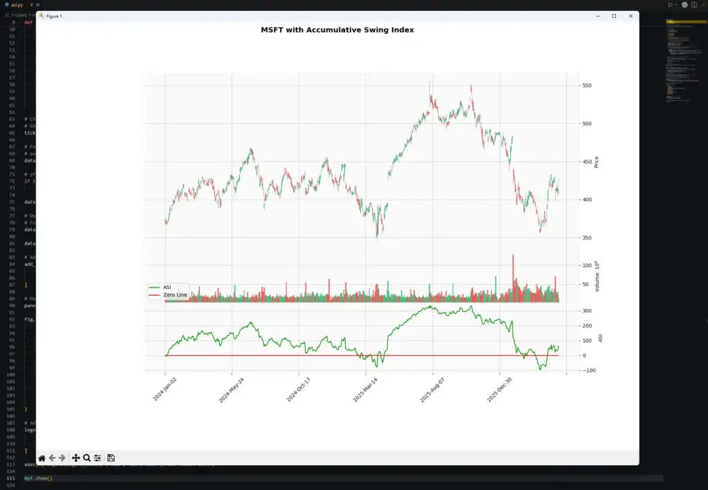
Finally, plot the candlestick chart, volume and ASI. The zero line is included so you can see when ASI is above or below zero.
# Additional plots for ASI and zero line
add_plots = [
    mpf.make_addplot(data["ASI"], panel=2, color="g", ylabel="ASI", secondary_y=False),
    mpf.make_addplot(pd.Series(0, index=data.index), panel=2, color="r", secondary_y=False),
]

# Main chart panel, volume panel, ASI panel
panel_sizes = (5, 1.5, 2)

fig, axes = mpf.plot(
    data,
    type="candle",
    style="yahoo",
    title=f"{ticker} with Accumulative Swing Index",
    ylabel="Price",
    addplot=add_plots,
    volume=True,
    volume_panel=1,
    panel_ratios=panel_sizes,
    figratio=(12, 8),
    figscale=1.1,
    returnfig=True
)

# Add a simple legend to the ASI panel
legend_lines = [
    Line2D([0], [0], color="g", lw=1.5),
    Line2D([0], [0], color="r", lw=1.5),
]

axes[2].legend(legend_lines, ["ASI", "Zero Line"], loc="lower left")

mpf.show()Save the file and run it in VSCode. It will fetch the data for the selected ticker, calculate ASI, and display a chart with price, volume and the ASI line.
If you have more than one Python version installed, make sure you install the packages into the same Python interpreter that VSCode is using. One safe way is to run python -m pip install rather than just pip install.
Because ASI is cumulative, the line begins accumulating from the start of the dataset you downloaded. That means your chart may not exactly match another charting platform that starts its ASI calculation from a different historical point or uses a different price-limit setting.
This example uses a 7% previous-close proxy for the limit move value. That lets us demonstrate the ASI calculation on a stock chart, but it is not an official exchange limit. If you apply ASI to a futures contract, use the relevant exchange or platform setting where available.
Because ASI is cumulative, the line starts accumulating from the first bar in the downloaded dataset. That means your chart may not exactly match a charting platform that uses a longer history or a different price-limit setting.
Applications
ASI is most useful when a trader wants a price-based confirmation tool rather than a simple momentum oscillator or volume indicator.
One common use is trendline confirmation. A trader may draw a trendline on the price chart and a comparable trendline on the ASI line. If price breaks out and ASI also breaks its own trendline, the move may carry more weight. If price breaks out but ASI does not confirm, the trader may treat the breakout with more caution.
ASI is often discussed in a futures context because the original formula includes a limit move value. That makes it more natural for markets where price limits and contract specifications are part of the trading framework. It can also be plotted on stocks or ETFs, as shown in the Python example above, but the price-limit setting then becomes an assumption rather than a true exchange-defined value.
For practical trading, ASI is best treated as one layer of evidence. It can help frame whether price swings are confirming a trend or warning of weakness, but it should not override market context, liquidity, news, support and resistance, volume, or risk management.
Comparing ASI with Other Trading Indicators
ASI is different from many popular trading indicators because it is based on the relationship between the current bar and the previous bar’s open, high, low and close. It does not use volume, and it is not designed to show overbought or oversold conditions in the same way as RSI.
That means ASI can sit alongside other indicators rather than replace them. For example, a trader might use ASI to confirm whether a breakout is supported by the swing structure, while using RSI to judge whether momentum is stretched, or MACD to assess broader trend momentum.
Volume indicators answer a different question. Accumulation Distribution Line and On-Balance Volume try to assess buying and selling pressure through volume. ASI does not do that. It is focused on price-swing behaviour.
A sensible combination might therefore be:
- ASI for trendline and swing confirmation;
- RSI for momentum and stretched conditions;
- ADL or OBV for volume confirmation;
- price structure for support, resistance, failed breakouts and risk levels.
The important point is not to stack indicators until the chart looks convincing. Each indicator should have a job. ASI’s job is to help judge whether price swings and breakouts are being confirmed by Wilder’s swing calculation.
Key Takeaways
- ASI was developed by J. Welles Wilder: The Accumulative Swing Index builds on Wilder’s Swing Index and accumulates one-bar swing values over time.
- ASI is price-based, not volume-based: It uses open, high, low and close relationships, but it does not use volume.
- The Swing Index comes first: ASI is the cumulative total of Swing Index values. SI measures one bar’s swing movement; ASI turns those values into a running line.
- The limit move value matters: The formula includes a price-limit value used to scale the Swing Index. For futures, use the proper exchange or platform value where available. For stocks and ETFs, any percentage-based value is only a proxy.
- ASI is mainly a confirmation tool: Traders often compare ASI trendlines with price trendlines to confirm or question breakouts.
- Divergence is a warning, not a trade signal: If price and ASI stop confirming each other, it may suggest weakness, but it should not be treated as an automatic buy or sell instruction.
- Coding ASI needs care: K, R and the price-limit value must be handled correctly. Small formula or operator-precedence mistakes can produce a different indicator.
- ASI should be used with other context: Support and resistance, trend, volume, market structure, liquidity and risk management all matter.
Further Reading
If you want to go back to the original source, Wilder’s New Concepts in Technical Trading Systems is the book where he introduced ASI alongside several other well-known technical indicators.
New Concepts in Technical Trading Systems by J. Welles Wilder, 1978.