Updated May 2026: This KAMA guide has been refreshed with clearer formula notes, trading-signal warnings, Python code improvements, and a more practical explanation of how the Efficiency Ratio adapts to noisy or trending markets.
Introduction
Kaufman’s Adaptive Moving Average, usually shortened to KAMA and labelled AMA on some charting platforms, adjusts its smoothing based on market behaviour. It is similar to an exponential moving average, except that it uses a scalable smoothing constant rather than a fixed one.
The key input is the Efficiency Ratio. This compares directional movement with volatility. When price moves cleanly in one direction, the Efficiency Ratio rises and the moving average responds more quickly. When price chops around in a congested range, the Efficiency Ratio falls and the moving average slows down.
That makes AMA useful as a trend-following and noise-filtering tool, but it is still a moving average. It can lag, it can whipsaw, and it should not be treated as a standalone trading system.
Key Takeaways
- Kaufman’s Adaptive Moving Average, or KAMA, is often labelled AMA on charting platforms.
- AMA adjusts its smoothing using the Efficiency Ratio, which compares clean directional movement with total market noise.
- When price moves efficiently in one direction, AMA responds more quickly. When price is choppy, AMA slows down.
- The common default setting is AMA(10, 2, 30): 10 bars for the Efficiency Ratio, a 2-period fast constant, and a 30-period slow constant.
- AMA is best used as a trend filter or noise filter, not as a standalone buy/sell system.
- Price crossovers and fast/slow AMA crossovers can be useful, but they still whipsaw in sideways markets.
- The Python example later in this article shows how to calculate and plot fast and slow AMA lines using recent market data.
Origins of the Adaptive Moving Average (AMA)
Perry J. Kaufman developed this adaptive approach as part of his wider work on trading systems and market efficiency. His aim was not simply to create another moving average, but to deal with a familiar trader problem: a moving average that is fast enough for trends is often too noisy in ranges, while a smoother average can be too slow when a real move begins.
Kaufman’s answer was to let the market decide how quickly the average should respond. If price is moving efficiently in one direction, the indicator speeds up. If price is chopping back and forth, it slows down.
Kaufman discusses adaptive methods and trading-system design in Trading Systems and Methods, now in its sixth edition. The Adaptive Moving Average remains useful because it directly addresses the old trade-off between responsiveness and noise.
Purpose and Design
The purpose of AMA is to reduce one of the main weaknesses of ordinary moving averages: the trade-off between speed and noise.
A fast moving average reacts quickly, but it can be chopped around in sideways markets. A slow moving average filters noise better, but it can lag badly when a new trend starts.
AMA tries to adapt between those two extremes. When price is moving cleanly in one direction, the Efficiency Ratio rises and the smoothing constant shifts closer to the fast setting. When price is moving sideways or erratically, the Efficiency Ratio falls and the smoothing constant shifts closer to the slow setting.
This makes AMA useful as a trend filter and noise filter. It can help traders judge whether price is moving efficiently enough to deserve attention, or whether the market is too choppy for a simple moving-average signal to be trusted.
It does not remove the usual moving-average problems. AMA can still lag, flatten too late, and produce false signals when price keeps crossing back and forth through the line.
How to Find Trading Signals with Adaptive Moving Average (AMA)
AMA is usually better as a trend filter than as a standalone trading signal.
The simplest use is trend identification. If price is above a rising AMA, the market may be in an improving trend. If price is below a falling AMA, the market may be in a weakening trend. If AMA is flat, the market may be too noisy or range-bound for a clean trend-following signal.
Some traders use price crossovers. A close above AMA can suggest that price is improving relative to its adaptive trend line. A close below AMA can suggest that price is weakening. This works best when the market is already trending. In a sideways market, price can repeatedly cross the line and create poor signals.
Another approach is to use two adaptive moving averages: a faster AMA and a slower AMA. When the faster line crosses above the slower line, it can suggest improving upside momentum. When the faster line crosses below the slower line, it can suggest deteriorating momentum.
The warning is that AMA does not make crossovers safe. It adapts better than a fixed moving average, but it can still whipsaw. Traders should treat AMA signals as one layer of evidence, not as an instruction to buy or sell.
A more cautious trader might use AMA to filter trades rather than trigger them. For example, only look for long setups when price is above a rising AMA, then use price structure, volume, support and resistance, or another indicator to decide whether the trade is worth taking.
The Efficiency Ratio in Simple Terms
The Efficiency Ratio is the heart of AMA.
It compares the distance price has travelled from point A to point B with the total amount of movement that happened along the way.
If price moves from 100 to 110 in a fairly straight line, the move is efficient. The Efficiency Ratio will be high, and AMA will respond more quickly.
If price moves from 100 to 110 but jumps up and down repeatedly on the way there, the move is less efficient. The Efficiency Ratio will be lower, and AMA will smooth more heavily.
In plain English:
High Efficiency Ratio = cleaner trend, faster AMA
Low Efficiency Ratio = more noise, slower AMA
Mathematical Construction
Kaufman’s Adaptive Moving Average is calculated in a similar way to an exponential moving average, but with one key difference: the smoothing constant changes as market conditions change.
A normal EMA uses a fixed smoothing constant. AMA uses a scalable constant, which is adjusted by the Efficiency Ratio.
1. EMA formula
First, the standard EMA formula is:
EMA_{\text{today}} = C \times (Price_{\text{today}} - EMA_{\text{yesterday}}) + EMA_{\text{yesterday}}or in plain text that would be:
EMA(today) = C × (Price(today) – EMA(yesterday)) + EMA(yesterday)
In this formula, C is the smoothing constant:
C = \frac{2}{N + 1}
in plain text that is:
C = 2 / (N + 1)
Here, N is the lookback period used to approximate a simple moving average. A shorter value of N gives a faster EMA. A longer value gives a slower EMA.
2. AMA formula
AMA uses the same basic structure, but replaces the fixed smoothing constant with a scalable constant, usually written as SC:
AMA_{\text{today}} = SC \times (Price_{\text{today}} - AMA_{\text{yesterday}}) + AMA_{\text{yesterday}}plain text:
AMA(today) = SC × (Price(today) – AMA(yesterday)) + AMA(yesterday)
That means today’s AMA moves toward today’s price by an amount controlled by SC. When SC is larger, AMA reacts more quickly. When SC is smaller, AMA moves more slowly.
3. Efficiency Ratio
ER = \left| \frac{Direction}{Volatility} \right|Plain text:
ER = | Direction / Volatility |
Direction is calculated as:
Direction = Price_{\text{today}} - Price_{\text{N bars back}}Plain text:
Direction = Price(today) – Price(N bars back)
Volatility is the sum of the absolute one-bar close-to-close changes over the same lookback period:
Volatility = \sum_{i=0}^{N-1} \left| Price_{t-i} - Price_{t-i-1} \right|Plain text:
Volatility = sum of absolute one-bar price changes over N bars
In simple terms, the Efficiency Ratio compares the direct distance travelled with the total amount of movement along the way.
If price moves from 100 to 110 in a fairly straight line, direction and volatility are similar, so ER is high. If price moves from 100 to 110 but jumps around heavily on the way, volatility is much larger than direction, so ER is lower.
High ER = cleaner trend, faster AMA
Low ER = more noise, slower AMA
4. Scalable Constant
The scalable constant uses the Efficiency Ratio to shift between a fast EMA constant and a slow EMA constant.
SC = \left[ ER \times (Fast - Slow) + Slow \right]^2
Plain text:
SC = [ER × (Fast – Slow) + Slow]²
The fast and slow constants are calculated like normal EMA smoothing constants:
Fast = \frac{2}{FastPeriod + 1}Plain text:
Fast = 2 / (Fast Period + 1)
Slow = \frac{2}{SlowPeriod + 1}Plain text:
Slow = 2 / (Slow Period + 1)
The common default settings are AMA(10, 2, 30):
- 10 bars for the Efficiency Ratio
- 2 bars for the fast EMA constant
- 30 bars for the slow EMA constant
Using those defaults:
Fast = \frac{2}{2 + 1} = 0.6667Plain text:
Fast = 2 / (2 + 1) = 0.6667
The final result is squared. This makes the smoothing constant much smaller when the Efficiency Ratio is low, helping AMA flatten out during noisy or congested markets.
When the market is trending cleanly, ER moves closer to 1 and AMA shifts toward the fast constant. When the market is choppy, ER moves closer to 0 and AMA shifts toward the slow constant.
That is the main point of the indicator: it tries to react quickly when price movement is efficient, and slow down when price movement is mostly noise.
Coding the Adaptive Moving Average
In this section we will code Kaufman’s Adaptive Moving Average in Python and plot fast and slow AMA lines on a candlestick chart.
The example uses free data from Yahoo Finance through yfinance, then plots the result with mplfinance. I am using VSCode, but the same code can be run in another Python environment if you prefer.
If you have more than one Python version installed, make sure you install the packages into the same Python interpreter that VSCode is using. One safe way is to run python -m pip install rather than just pip install.
Step 1: Create a new Python file
Open VSCode and create a new Python file. Save it as something like kama_chart.py or ama_chart.py.
We will build the script in four stages: importing libraries, defining the AMA function, downloading price data, and plotting the chart.
Step 2: Import the necessary libraries
import pandas as pd
import numpy as np
import yfinance as yf
import mplfinance as mpf
import matplotlib.lines as mlines
import matplotlib.pyplot as pltIf these libraries are not already installed, open a terminal in VSCode and install them into the same Python environment you are using to run the script.
python -m pip install pandas numpy yfinance mplfinance matplotlibStep 3: Define the AMA calculation function
def calculate_ama(price, fast_period=2, slow_period=30, er_period=10):
    direction = price - price.shift(er_period)
    volatility = price.diff().abs().rolling(er_period).sum()

    er = (direction.abs() / volatility).replace([np.inf, -np.inf], 0).fillna(0)

    fast_sc = 2 / (fast_period + 1)
    slow_sc = 2 / (slow_period + 1)
    sc = (er * (fast_sc - slow_sc) + slow_sc) ** 2

    ama = pd.Series(index=price.index, dtype="float64")

    # Seed the series with the first available price
    ama.iloc[0] = price.iloc[0]

    for i in range(1, len(price)):
        if pd.isna(sc.iloc[i]):
            ama.iloc[i] = ama.iloc[i - 1]
        else:
            ama.iloc[i] = ama.iloc[i - 1] + sc.iloc[i] * (price.iloc[i] - ama.iloc[i - 1])

    return ama
The function first calculates direction, volatility and the Efficiency Ratio. It then converts the Efficiency Ratio into a smoothing constant and uses that value to update the moving average one bar at a time. When price movement is efficient, the smoothing constant rises. When price movement is noisy, it falls.
Step 4: Download data and calculate the AMAs
Here we download recent Apple data and calculate two adaptive moving averages. The first uses the common AMA(10, 2, 30) settings. The second uses a longer Efficiency Ratio period, so it adapts more slowly.
ticker = "AAPL"

df = yf.download(
    ticker,
    start="2024-01-01",
    auto_adjust=False,
    progress=False
)

# yfinance can sometimes return MultiIndex columns, so flatten them if needed.
if isinstance(df.columns, pd.MultiIndex):
    df.columns = df.columns.get_level_values(0)

df = df.dropna()

df["Fast AMA"] = calculate_ama(df["Close"], fast_period=2, slow_period=30, er_period=10)
df["Slow AMA"] = calculate_ama(df["Close"], fast_period=2, slow_period=30, er_period=30)Step 5: Plot the Data
Finally, plot the candlestick chart with volume and the two AMA lines.
fast_ama_line = mpf.make_addplot(df["Fast AMA"], color="b", width=1.5)
slow_ama_line = mpf.make_addplot(df["Slow AMA"], color="r", width=1.5)

fast_dummy_line = mlines.Line2D([], [], color="blue", linewidth=1.5, label="Fast AMA")
slow_dummy_line = mlines.Line2D([], [], color="red", linewidth=1.5, label="Slow AMA")

fig, axes = mpf.plot(
    df,
    type="candle",
    style="yahoo",
    title=f"{ticker} with Adaptive Moving Averages",
    ylabel="Price",
    addplot=[fast_ama_line, slow_ama_line],
    figratio=(12, 7),
    figscale=1.1,
    volume=True,
    returnfig=True
)

axes[0].legend(handles=[fast_dummy_line, slow_dummy_line])

plt.show()Once you have pasted all Python sections into your Python file in VSCode, you can save and run the file by clicking on the green play button in the top-right corner or by pressing Ctrl+Alt+N. You should see a candlestick chart of AAPL’s closing prices along with the fast and slow AMAs that looks like mine shown here:
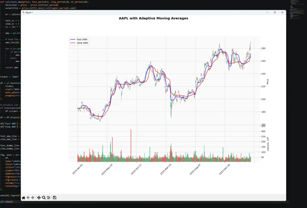
The faster AMA should react more quickly to trend changes, while the slower AMA should filter more noise.
The chart will not be a trading system by itself. It simply shows how the adaptive moving average changes its speed as the Efficiency Ratio changes.
Pros and Cons of Adaptive Moving Average (AMA)
Like any moving average, AMA has strengths and weaknesses. Its main advantage is that it tries to adapt to the market instead of using one fixed speed all the time.
Pros of AMA
- Adapts to market conditions: AMA becomes more responsive when price is moving efficiently and slows down when price is noisy or range-bound.
- Helps filter choppy price action: In sideways markets, AMA can reduce some of the false movement that would affect a faster fixed moving average.
- Useful as a trend filter: Traders can use AMA to decide whether the market is trending cleanly enough to consider trend-following setups.
- Easy to plot and compare with price: AMA sits directly on the price chart, so it is simple to compare price action with the adaptive trend line.
- More flexible than a fixed moving average: Because the smoothing constant changes, AMA can behave more like a fast average in clean trends and more like a slow average in noisy markets.
Cons of AMA
- Still a lagging indicator: AMA reacts to price behaviour. It does not predict the future.
- Can still whipsaw: Although AMA adapts better than a fixed moving average, it can still produce poor signals when price repeatedly crosses the line in a range.
- More complex than SMA or EMA: The Efficiency Ratio and scalable constant make AMA harder to understand and code than a standard moving average.
- Parameter choices matter: Changing the Efficiency Ratio period, fast period or slow period can materially change the line. A setting that works well on one market may not suit another.
- Not a complete trading system: AMA can help define trend conditions, but entries, exits, stops, position sizing and market context still need to be handled separately.
Application
AMA is most useful when a trader wants to separate cleaner trends from noisy price movement.
A simple application is to use AMA as a trend filter. If price is above a rising AMA, a trader may prefer long setups. If price is below a falling AMA, a trader may prefer short setups. If AMA is flat, the market may be too choppy for a clean trend-following approach.
Another use is to compare a faster AMA with a slower AMA. The faster line reacts more quickly to changes in price behaviour, while the slower line filters more noise. A crossover between the two can highlight a possible shift in trend, but it should not be treated as a mechanical buy or sell instruction.
AMA can also help with breakout trading. If price breaks out of a range and AMA begins to turn in the same direction, that can support the idea that the move is becoming more efficient. If price breaks out but AMA remains flat, the breakout may deserve more caution.
For discretionary traders, AMA can be useful as a “market quality” filter. A steep, rising AMA suggests cleaner upside movement. A flat or repeatedly crossed AMA suggests noise, indecision or poor trend quality.
The important point is to give AMA a specific job. Use it to judge trend condition, filter setups or compare clean movement with noise. Do not ask it to replace trade planning, risk management or awareness of news and market structure.
Conclusion
Kaufman’s Adaptive Moving Average is useful because it addresses a real moving-average problem: fast averages react quickly but get chopped around, while slow averages are smoother but often late.
AMA tries to adapt between those extremes by using the Efficiency Ratio. When price movement is clean, it speeds up. When price movement is noisy, it slows down.
That makes it a useful trend and noise filter, but not a complete trading system. The best use is usually to combine AMA with price structure, support and resistance, volume, news context and sensible risk management.
If you use AMA in your own trading, pay attention to when it helps and when it fails. The indicator’s real value is not just in the line itself, but in whether it helps you avoid poor trend signals in messy markets.
Further Reading
“Trading Systems and Methods” Perry J Kaufman, (Wiley Trading) 6th Edition, 2019